Journal of the Operational Research Society

1. Introduction

IFRS9 is an international accounting standard that requires a lender to predict the expected cash flow and hence any loss from a loan if the risk of its default changes. All large banks were required to implement this regulation from January 2018. CECL is a similar regulation applicable to lenders of all sizes in the US. Between them they apply to all large banks globally. Whilst there is a large literature on the the accounting principles underlying these regu- lations there are few papers that address the appro- priate modelling techniques to use and lenders have found the modelling of such losses challenging. The aim of this paper is to propose a new method to model expected losses over the lifetime of an account which will yield more accurate predictions of losses than established methods and that will enable the analyst to make predictions both in the short-term, that we define as over a 12-month hori- zon, and over a longer-term. The method also gives point in time estimates, as required by IFRS 9 and useful in CECL.

Finalised in 2014, IFRS 9 makes requirements according to whether or not a loan experiences a significant increase in the risk of default since initial recognition. For a non credit impaired loan, fore- casts of expected losses over the ensuing 12 months are required. If there has been, or is expected to be a significant increase in credit risk after the first 12 months, then the bank must predict the lifetime expected credit losses for each account with interest computed on a gross basis. This is known as a Stage 2 credit loss forecast. If there is a credit impairment then expected lifetime credit losses must be com- puted and interest treated on a net basis. In each case expected losses are to be computed as the prob- ability of default in a month multiplied by the cash shortfalls in the event of default. Expected losses in each month in the future are to be discounted. CECL was implemented in the US in 2016 and required a lifetime expected loss to be computed for all loan accounts without use of stages.

Accurate prediction of expected losses from a loan portfolio is a vitally important challenge faced by lenders. The expected losses determine the provi- sions that each lender needs to charge borrowers and to retain as a form of capital to protect deposi- tors in the event of the lender becoming bankrupt. So accurate prediction impacts borrowers in terms of the interest rates they are charged. It is also important for depositors who receive some degree of protection, and it impacts shareholders whose return on equity may be reduced if greater provi- sions are retained as accrued profits. Clearly banks wish to compute the most appropriate amount of provisions given the riskiness of the loans but not an excessive amount that unnecessarily reduces the ability of the lender to make loans.

One can consider models that may be used to predict losses for a portfolio as a whole, by segments of a portfolio, or at the level of an individual account. In the first case the literature discusses two methods to compute expected losses of a loan port- folio in the event that the credit risk increases (see for example Brunel (2016) or Siddiqi (2012)). One method is to use roll rates. A roll rate may be com- puted in terms of balances in which case it is defined as the aggregate value of balances outstand- ing in a state of delinquency at time t divided by the balance in the immediately lower delinquency state in the previous time period. It is computed for each number of months delinquent. The lifetime loss for the portfolio is then defined as the sum of the balances that reach a default state, such as six months delinquent, where the latter is the balance at the end of the previous period of accounts that are 5 payments behind times the roll rate from the state of being 5 behind to 6 behind.

Various authors have noted Brunel (2016) and McPhail and McPhail (2014) that roll rates trad- itionally assume past rates remain valid into the future, or they may be forecast using an ARIMA model, but they do not include any explanatory fac- tors that may allow their value in the future to be predicted in a systematic way if such predictors change. However, best practice at financial institu- tions often model the time series of the roll rates with transformations of macroeconomic factors. That approach was followed by Breeden (2018) and is followed here. Still roll rates do not capture fluc- tuations due to changes in the credit quality of the loans originated or the maturing of loans from origination.

A second portfolio method is the so called “vintage” or “Age-Period Cohort” model Mason and Fienberg (1985) and Yang and Land (2014). In this approach aggregate default rates are decomposed into the influence of the time a group of loans was started (originated), the time since the loan has been opened (age or duration time) and factors that influence the probability of default and that vary over time like macroeconomic factors (see Glenn, 2005; Breeden, 2010; McPhail & McPhail, 2014).

Turning to account level models one may con- sider a state transition model. Here the probability that an account transits from one state of delin- quency to another is predicted. The expected life- time loss can be computed as the probability of default weighted by possible loss over the expected or defined life of a loan. There are several method- ologies for making these predictions. In one, the probability that an account will transit from being in one specific state, j, to another, k, between time t and t þ 1 is estimated using a cumulative posterior probability model in terms of the value of the state the account is in in previous periods, lagged macro- economic variables and the lagged age of the loan. In this approach the regression coefficients are spe- cific to the state of the account at t and assumed to be the same no matter which destination state the account transits to (see for example Malik and Thomas (2012)). Published studies Malik and Thomas (2012) using this approach use a behav- ioural score as the state indicator, which has been estimated from some other model. This may be problematic if what the analyst is after is a state in terms of days past due because the behavioural scor- ing model may not be accurate and because a behavioural score does not translate directly into a delinquency state. The model of Malik and Thomas also omits covariates presumably because in some way they are included in the behavioural model, but it means one cannot predict transition probabilities for new cases without having the behavioural model score in previous periods. There may also be estima- tion issues. The model implicitly relates the transi- tion probabilities to a set of covariates in a behavioural model, but the final model is estimated in two stage models with errors at both stages, yet the error distribution of the implicit model has not been specified.

Another method is to estimate a multistate inten- sity model where the probability of transiting between state j and k is specified as a hazard model where the set of regression parameters is specific to the transition rather than to the initial state. This approach is followed by Lando and Skdeberg (2002) for corporates and by Leow and Crook (2014a) and Djeundje and Crook (2018). The latter included a frailty parameterisation and macroeconomic varia- bles as well application and behavioural variables. These models enable probabilities of cure as well as advanced delinquency. Published applications of this methodology to credit risk have defined states in terms of days past due and estimated the coeffi- cients in one step.

A multistate intensity model would enable an analyst to predict losses arising from each transition into each sate, for example when a payment is missed but the account does not default. But from a practitioner point of view such models are relatively complex and a simpler method that still enables the prediction of losses in each month in the life of a loan may suffice. Hazard models of the probability that an account will move into the default state in the next month, given that it has not done so before is an example of such a method. There is a rapidly growing literature on the application of survival models to the probability of credit default. Again there are several approaches. One is to use applica- tion, and lagged bahavioural and macroeconomic variables as predictors. Recent literature for retail credit default includes Banasik et al. (1999) and Stepanova and Thomas (2002) (both omit macro- economic variables) and Bellotti and Crook (2012), Bellotti and Crook (2009), Bellotti and Crook (2013); and Djeundje and Crook (2018) that include macroeconomic variables. Many recent papers have also explored using machine learning methods to estimate the components of hazard models Biganzoli et al. (1998) and Faraggi and Simon (1995) or com- bine multiple models Hothorn et al. (2006); Hothorn et al. (2004); and Ishwaran et al. (2008). Wang et al. (2019) provide a thorough survey of methods to date.

Others have explored the use of time varying coefficients in a Cox proportional hazards frame- work. This involves having both time-varying risk covariates and time-varying sensitivities (Sargent, 1997; Tian et al., 2005). Djeundje and Crook (2019) tested this approach on data through the 2019 Global Financial Crisis and found it to be effective at capturing the shifts in consumer behaviour quickly enough to predict future performance.

Empirical evidence and practitioner experience of using the roll rate and transition probabilities approaches is that they are relatively accurate when predicting over 12 months but less accurate when predicting over longer time horizons (see for example FDIC (2007) and McPhail and McPhail (2014)). Vintage models such as age-period-cohort models are accurate for aggregate forecasting over long horizons, but can be quite inaccurate in the beginning as they do not consider account-level details such as delinquency. When predicting losses for IFRS9 and CECL, some accounts will have only a short remaining duration while others require a long forecast horizon. Therefore, we need model accuracy over both short and long forecast horizons.

In this paper we propose a variant of the hazard model approach that is more accurate than either roll-rates or transition models over both the short term and as good as vintage models for long term forecasts. Such predictions are necessary across all loan types. This technique allows for time-varying covariates, as many other methods do. In theory it could also be complimentary to multistate methods and techniques using time-varying coefficients. However, the primary goal is to solve a different, also important problem of optimising the use of available information at the start of the forecast to make predictions out to different forecast horizons in an internally consistent framework.

We parameterise the model using a combined Fannie Mae and Freddie Mac conforming mortgage portfolio and demonstrate its relative accuracy in comparison to roll rate, vintage, and state transition models. Thirty-year term, fixed interest rate mort- gages were selected for the test, because they are an important asset class and a worst-case for loss reserves under CECL. The data provides loan-level performance detail with commonly considered ori- gination and behavioural factors.

This paper makes the following contributions to the literature. First we present a new variant of a hazard model to predict the probability of default in each month of the life of an account. Our innov- ation is to include a thorough investigation of the role of past delinquency of various degrees as a pre- dictor. Second our proposed model is tested on a large sample of 30 year conforming mortgage accounts. Third our tests show that our proposed model makes more accurate predictions than either roll rate methods or a state transition method using scoring and macroeconomic factors. Fourth we show that this is because of the enhancement of predictive power of lagged delinquency terms and we show that the marginal effects of lagged delin- quency varies systematically with the lag, in the same way, for each type of delinquency.

Our paper is structured as follows. Following this introduction we explain the model. Section three describes the application data and the fourth section presents the results of this application. In sections five and six we compare the predictive accuracy of the model to roll rate, vintage and state transition models. The final section concludes.

2. Model description

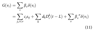
The model development begins with concepts from Age-Period-Cohort (APC) models Glenn (2005); Mason and Fienberg (1985); and Ryder (1965), where loan performance can be described as a com- bination of three functions. This is a panel model with time varying variables. One function is loan repayment performance as a function of age of the loan, FðaiÞ where a denotes age of a loan. This rep- resents a lifecycle pattern of performance over the life of a loan. A second function represents perform- ance as a function of origination date, GðviÞ where vi is the origination date for account i. Loans origi- nating around a similar date, would be expected to have been of a similar maximum level of risk and a pool of such loans to be of similar risk composition. This relationship is often referred to as a “vintage” effect. The third function represents performance as a function of calendar date, HðtiÞ where ti denotes calendar time for account i. This relationship relates performance to exogenous factors such as macro- economic conditions. The functions can be parame- terised in many ways, but the most general form is to use a set of dummy variables, one for each value of the relevant time variable. Each dummy variable is represented as dðuÞ where

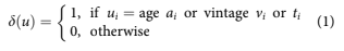
and i denotes case i.

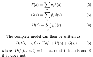
The coefficients aa, bv, and ct need to be esti- mated. Because only one overall intercept term may be estimated, the estimates are constrained so that

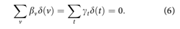
Because of the relationship t 1⁄4 v þ a, an assump- tion must be made about how to remove the linear specification error. Consistent with earlier work (see Appendix in Breeden and Canals-Cerda (2018)), this is accomplished using an orthogonal projection onto the space of functions that are orthogonal to all lin- ear functions. The coefficients obtained are then transformed back to the original specification.

Traditional APC or Bayesian APC estimators Schmid and Held (2007) process vintage aggregate data. But in the current work we are interested in a loan-level estimator.

Default is modelled conditioned on the account not having previously closed. Any account closure that is not a default is called attrition or prepay- ment. To capture this effect, a parallel equation for modelling atttrition is employed.

Although the structure is the same as for the default model, the functions FattðaÞ,GattðvÞ, and HattðaÞ will be different, because the drivers of attrition perform- ance will be different from those for default.

By using dummy variables for vintage in the APC for- mulation, the model can measure credit risk but not explain it. Therefore, to enhance the usefulness of the model and to better predict default, information collected at the time of application is added to the formulation.

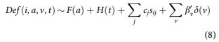
where sij are the available attributes at origination for account i. Such attributes include origination FICO score and origination loan-to-value (LTV), for example. The cj are the coefficients to be estimated. Vintage dummies are still included, but with new coefficients b0 v such that for a given v,

This approach was used to study root causes of the 2009 US Mortgage Crisis (Breeden & Canals- Cerda, 2018).

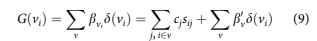
We know from the work by Holford (1983) that once the constant and linear terms are appropriately incorporated, the nonlinear structure for F, G, and H is uniquely estimable. The treatment of the constant and linear terms described above satisfy this condition, meaning that the vintage aggregate structure G(v) must be equivalent to the aggregate credit risk for the accounts i in that vintage, as shown in Equation 9. Said differently, the estimates of F(a) and H(t) do not change with the loan-level attribution of credit risk in Equation 8. Of course, Equation 8 will be more accur- ate at the account level than Equation 5 that only has a vintage level credit risk measure.

Note that this loan-level version of an APC model is identical to a discrete time survival model where a dummy variable is used for each value of age and time. Therefore, the same parameter estima- tor is used here as for a discrete time survival model. Notice also that this discrete time survival model is just a panel model with age and time fac- tors added beside the usual explanatory factors.

To achieve the short term accuracy of roll rate and state transition models, we need to incorporate delin- quency in the model. This creates complications in any APC or survival model structure, because delin- quency is also a function of the age of the account and the economic and portfolio management environ- ment and therefore correlated to F and H that appear in Equations 5 and 8. Equation 10 provides the gen- eral structure including delinquency.

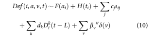
where Dk iðtLÞ are again indicator variables, one for each possible delinquency state leading up to default.

If all parameters in Equation 10 are estimated simultaneously, F and H will likely change from the values in Equation 8 because of the multicolinearity with the dkDk iðtLÞ: An alternative that will be explored here is to constrain the estimation of the dk such that F and H are retained from the estimate in Equation 5. The result would be that

Whenever time-varying predictive factors are used, referred to in the lending industry as behav- ioural factors, one faces the question of how to extrapolate those factors. The question becomes acute in lifetime loss forecasting where long range extrapolations would be required. However, fore- casting the delinquency factors above is comparable in difficulty to forecasting default. Since the primary drivers of future delinquency would again be some measure of age and time effects, little new informa- tion is gained beyond that already available in the default equation.

Therefore, the current approach is to create a set of models using the structure of Equation 10, each with different lags on the behavioural factors. If a model uses only behavioural factors with lags as small as L, then that model can be used to forecast L steps into the future without the need to forecast the input factors. Thus, if we have a set of N mod- els, one each for L l for l 2 1⁄21, N, then a full set of forecasts out to N periods into the future can be created without forecasting the input factors. The hope is that as N becomes large, the coefficients cj and dk approach limiting values such that forecasts can continue to be generated for forecast horizons greater than N, again without forecasting the input factors.

If we define the model by the minimum allowed lag for the behavioural factors,

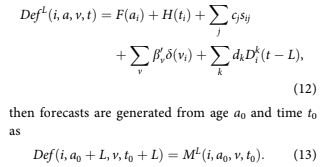
DefL is a kind of discrete time survival model Bellotti and Crook (2013); Cox (1972); and Tutz and Schmid (2016), one such model for each fore- cast horizon (value of L).

A parallel approach is used for modelling account attrition/pay-off. To get to charge-off balance, add- itional models of exposure at default (EAD) and loss given default (LGD) would be required. Those are not considered here, since they are independent questions potentially requiring different model- ling techniques.

3. Data

3.1. Mortgage data

Data was obtained from Fannie Mae and Freddie Mac for 30-year, fixed-rate, conforming mortgages.

The data contained de-identified, account-level information on balance, delinquency status, pay- ments, pay-off, origination (vintage) date, origin- ation score, postal code, loan to value, debt to income, number of borrowers, property type, and loan purpose. Risk grade segmentation was defined such that Subprime is less than 660 FICO, Prime is 660 to less than 780, and Superprime is 780 and above.

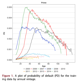
The data in this study represents more than $2 trillion of conforming mortgages. The data made available by Fannie Mae and Freddie Mac is a large share of their respective portfolios, but not the entirety. Figure 1 shows the historic default rate aggregated by annual vintage.

3.2. Macroeconomic data

As part of the government’s implementation of the Dodd-Frank Stress Test Act (DFAST), the Federal Reserve Board regularly releases Base, Adverse, and Severe scenarios for a set of macroeconomic factors. Since these factors and scenarios have become industry standards, this study has focussed on the use of these factors for incorporating macroeco- nomic sensitivity. For mortgage modelling, the most interesting are real gross domestic product (GDP), real disposable income growth, unemployment rate, CPI, mortgage interest rate, house price index, and the Dow Jones stock market index (DJIA).

4. Model estimation

Model estimation occurs in three stages. The first step is to apply an APC decomposition to estimate the lifecycle, environment, and vintage quality

functions. During that stage, methods such as described in Breeden and Thomas (2008) may be applied to achieve linear trend stability. The second step is to include those lifecycle and environment functions into Equation 12, and estimate Equation 12 as a logistic regression, one estimation for each forecast horizon, L. The third step is to estimate a time series model of the environment function using macroeconomic factors.

4.1. APC decomposition

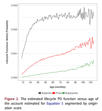
A Bayesian APC algorithm was used to estimate the functions in Equation 5. The estimated PD lifecycle versus age of the account, F(a), is shown in Figure 2. The estimated relationship between PD and vin- tage is shown in Figure 3. The estimated relation- ship between PD and calendar date, H(t) is shown in Figure 4. In all three figures the functions are segmented by credit quality: subprime, prime or superprime.

The lifecycles include the overall constant term for the analysis and are transformed to probability of default per month so that they may be under- stood more intuitively than on a log-odds scale. They show that the PD of the subprime segment rises faster relative to account age and to a higher level compared to the PD of the superprime seg- ment that rises gradually and always at a much lower level.

The PD vintage functions in Figure 3 are mean- zero and on a log-odds scale. They show that the credit cycle was most severe for the superprime seg- ment. Proportionally, the 2006–2008 vintages were worst for superprime even though loss amounts

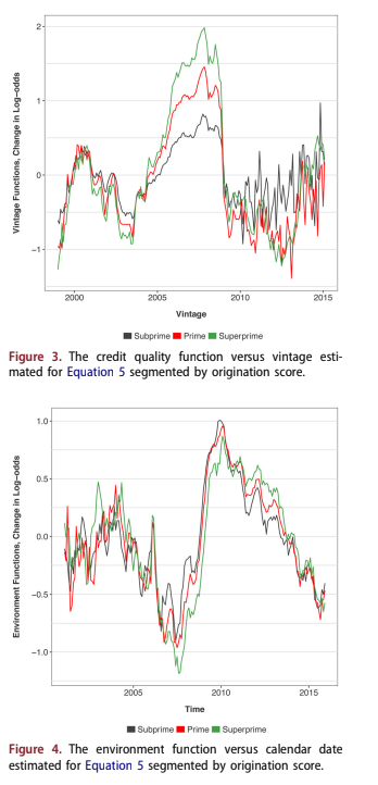
were smaller than for subprime. After 2010 the esti- mates for each vintage are much more volatile, because those vintages have far fewer cases.

The PD calendar time functions in Figure 4, also on a log-odds scale, show that the macroeconomic impacts were nearly equivalent across all risk bands on a proportional basis. Since these risk bands are all for conforming mortgages, they do not include the most extreme non-conforming loans. Differences may arise when taken to those extremes.

4.2. Loan-level coefficients

The discrete time survival model represented by Equation 12 was estimated separately for each credit

risk segment and each forecast horizon. Through testing, the model coefficients were found to stabil- ise by horizon 12, so no further coefficients were estimated. The coefficients for horizon 12 were applied to all horizons greater than 12.

A separate model was created to predict at the time of origination that did not include any behav- ioural factors such as delinquency since no values of behavioural factors exist in the first few months after account opening. The origination model was applied to all accounts less than 6 months on book at the start of the forecast.

The estimation of Equation 12 takes the esti- mated parameters for the lifecycle function, F(a), and the environment function, H(t), as fixed, so the coefficients cj, dk, and b0 v0 are estimated to replace the vintage effects in the PD model. The result is a

set of estimations, one for each value of L and risk segment. Vintage dummies, b0 v0, are included as possible explanatory factors in order to capture adverse selection or consumer risk appetite as was observed by Breeden and Canals-Cerda (2018).

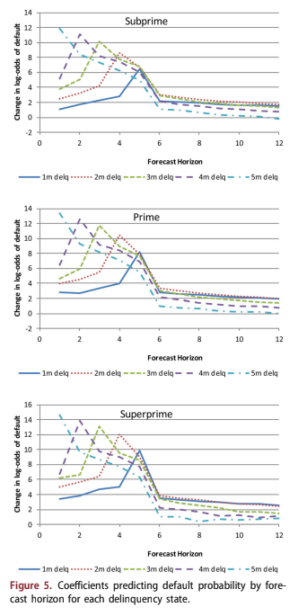
Figures 5 and 6 graph the coefficients dk and cj, respectively, one for each lag and credit quality. Although estimated independently, Figure 5 by risk grade show nearly identical structure. Each line is the probability of default with forecast horizon for accounts in a certain delinquency state at the start of the forecast. Default is either contractual default at 6 months delinquency or caused by non-contrac- tual reasons such as bankruptcy, fraud, or deceased.

Because the coefficients are functions of the fore- cast horizon, the importance to the forecast depends

upon how far into the future one is trying predict. Figure 5 is a good example of this.

When trying to predict one month forward, severe delinquency is the strongest predictor of default. An account that is 2 months delinquent at the start of the forecast has the greatest risk of default at horizon 4. For all delinquency states, the predicted value declines dramatically beyond 6 months into the future, because delinquent accounts will most likely have either cured or defaulted by then. In fact, the most severely delin- quent accounts (5 months delinquent in this ana- lysis) are less likely to default at horizon 6 than a less delinquent account. Presumably, this is because any 5-month delinquent accounts that are still active by 6 months into the future must have cured and therefore are not such a severe default risk.

All of the delinquency coefficients are measured relative to non-delinquent accounts, which are thus assigned a coefficient of 0. This means that any delinquent account is more risky than a non-delin- quent account, but the relationship for delinquent accounts is highly nonlinear. If only contractual default were considered, then the coefficients for all delinquency states would be 0 until enough months had elapsed for the account to move from the cur- rent state to default, defined as 6 months delinquent.

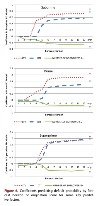
Figure 6 shows the coefficients for some of the other variables in the scores. Note that in the first few months of the forecast, the other candidate vari- ables make almost no contribution to the forecast – delinquency is everything. As the predictive value of delinquency diminishes around horizon 6, the other factors take over. By horizon 12, the coefficients have almost converged to the values that appear in the origination score, meaning that for long-range forecasting, origination information still dominates behavioural information. This is probably not true for credit cards, for example, where the transactor/ revolver distinction is critical for the entire forecast.

The model is already segmented by FICO, so it does not appear directly in the explanatory factors. Although tested, it was no longer significant beyond the initial segmentation.

The importance of current delinquency decays rapidly with time. However, as delinquency loses value, other measures such as loan to value ratio (LTV), debt to income ratio (DTI), and number of borrowers take over. These coefficients are shown in Figure 6. Unlike delinquency, the information con- tent of these three origination variables is stable for long horizons. The coefficients do not return to the origination model values, because behavioural varia- bles like delinquency provide some information. The ability to adapt to the information decay rate of each variable is what provides the combination of short-term and long-term forecast accuracy.

In addition to the factors shown here, the PD models for subprime and superprime also included origination balance. The model for prime included origination balance, loan purpose, and occu- pancy status.

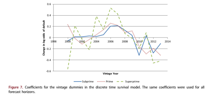
Figure 7 shows the coefficients for annual vintage dummy variables. Note that the Superprime line is the most volatile, because the fewest number of defaults were available for the modelling. Overall, these agree with the results of a previous study on consumer risk appetite Breeden and Canals-Cerda (2018), showing that the 2005–2008 vintages had significant residual credit risk that was not captured by the available scoring factors.

4.2.1. Model fit tests

Because the multihorizon model uses 12 separate regressions for the behavioural model plus one for the origination model, the model fits and

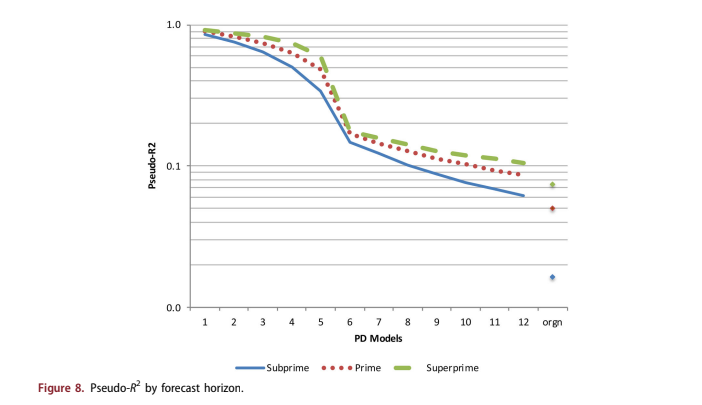
discrimination tests of each model were measured sep- arately. Figure 8 shows the coefficients for pseudo-R2, defined as 1 Residual Deviance = Null Deviance: For short forecast horizons, the pseudo-R2 is very high. It falls dramatically as delinquency information decays and approaches the pseudo-R2 for the origin- ation model as the forecast horizon becomes large.

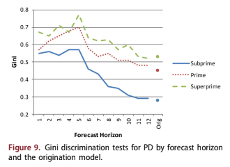
Discrimination ability was measured by the Gini coefficient, which was again computed separately for each forecast horizon and the origination model, Figure 9. This shows that discrimination ability is strong through the first 6 months of the forecast and then again descreases towards the origin- ation values.

4.3. Macroeconomic modelling

The macroeconomic model was created as a time series model of the environment functions in Figure4 using transforms and lags of macroeconomic fac- tors Breeden and Thomas (2008). The macroeco- nomic model is used only to translate macroeconomic scenarios into scenarios of the environment function. In the current context, the primary purpose is to provide a fair comparison to alternative methods where all models can be given the same input macroeconomic factors.

The transformations were optimised individually via an exhaustive search of the lags and transform widths. The optimised transforms were then com- bined in all possible combinations up to a max- imum of five factors to find the one that had the best adjusted R2 while still having the intuitively correct sign for the factor and significant p-values using a Newey-West robust estimator Newey and West (1987). Five was considered to be a stopping point, since no five-factor models survived the above constraints due to loss of significance.

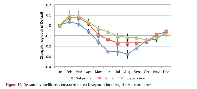
The macroeconomic modelling was done concur- rently with estimating seasonal effects. The seasonal- ity coefficients are shown in Figure 10 along with confidence intervals. All of the other coefficients in the loan-level and macroeconomic analysis were tested to ensure that the p-values were significant. However for seasonality, the zero level was arbitrar- ily set to January, so the monthly coefficients should not be tested separately for significance. Instead, it must be viewed as a function to determine if the range of variation is significant relative to the confi- dence intervals, which it is.

The macroeconomic models are summarised in Table 1. The factors are listed along with the trans- formation used, lags applied, and the width of the

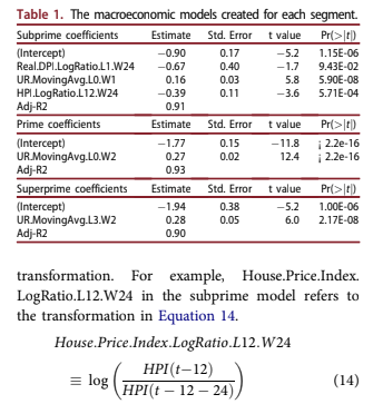
Although all the consumer-related factors in the DFAST scenarios were considered, the ones chosen through this automated process were intuitively obvi- ous: unemployment rate (UR), house price index (HPI), and disposable personal income (DPI). DPI and HPI were only considered with the log-ratio transformation demonstrated in Equation 14 in order to ensure stationarity. The proper transformation of UR is not clear, because past studies have shown that both levels and changes in UR can be predictive. In this case, both were tested but moving averages were found to be optimal.

5. Alternate approaches

To provide a means of comparison, several other stand- ard models were estimated on the same data set. For brevity, the full estimations for those models are not shown, but a summary description is provided for each and the results are included in the forecast comparisons. We wish to compare the predictive accuracy of the mul- tihorizon model with alternative methodologies.

5.1. Vintage models

The multihorizon survival model developed here can be viewed as an extension of age-period-cohort (vintage) models. Therefore it is reasonable to ask what would happen if the analysis stopped with aggregate vintage modelling instead of going to loan level modelling.

The vintage models for probability of default and probability of attrition/pay-off were used to predict the expected number of defaults each month for each vin- tage. Balances were not modelled, since different mod- els are often used to model exposure at default and loss given default. The test here is only of the probabil- ity of default and probability of attrition models.

The vintage model results shown below use the life- cycle and environment from Figures 2–4, but re-esti- mate the vintage coefficients at the beginning of each test period. This is only a partial out-of-sample test, because the training data would be too short to create a stable estimate of the lifecycle and macroeconomic model without at least one full economic cycle.

5.2. Roll rate models

Roll rate models are another aggregate modelling approach FDIC (2007), and one that has been in use in lending since at least the 1960s. Balance roll rates are the most commonly used, because they are the most simple. However, to create a fair compari- son to the default account forecasts for the other models, account roll rates are used here, defined as

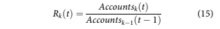
month t, and RkðtÞ is the net roll rate. R6 RD, which is the roll to default.

To capture account pay-offs, an additional payoff rate, Rp, is required.

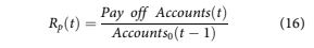
These roll rates are modelled historically with macroeconomic factors using the same kind of pro- cess described in Section 4.3, wherein the roll rate time series are modelled with transformations of the same macroeconomic factors listed previously. Again, a grid search over possible lags and windows for the transformations was used, and all models must satisfy criteria related to significance and the sign of the relationship.

To create forecasts, the following equations were used.

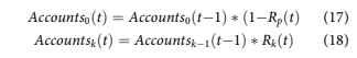
The final lifetime loss is calculated by summing the default accounts until all Accountsk reach 0. Note that in these formulas, no new accounts are included, so Accounts0 should decrease with time.

5.3. State transition models

State transition models Bangia et al. (2002); Djeundje and Crook (2018); Israel et al. (2001); Leow and Crook (2014b); and Thomas et al. (2001) are the loan-level equivalent of roll rate models. Rather than modelling aggregate movements between delinquency states, the probability of transition is computed for each account. The states considered are current (not delinquent), delinquent up to a maximum of five months delinquent, default, and pay-off. Account transition probabilities are modelled. For an account i in state j at time t, the transition probability to state k 2 1⁄20:::5, D, P is given as

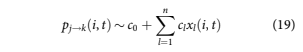
Each transition with sufficient data was modelled with a separate logistic regression to estimate coeffi- cients cl for predictive factors xlði, tÞ: This includes all state transitions pj!k for which kj 2 1⁄22, 1, 0, 1, meaning two forward transitions and one backward transition. Transitions to other states that were too rare for modelling (kj 62 1⁄22, 1, 0, 1) were included as constant probabilities. Also modelled were all transitions pi!0,sj!D, and sj!P, where D and P refer to default and prepayment. As noted before, default can occur from any delinquency state because of bankruptcy, fraud, deceased, or abandonment.

The transition matrix is close to diagonal because monthly transitions are being modelled. Transitions over longer periods, like quarters or years, would cause a greater spread in the transition matrix.

The regression factors xlði, tÞ in Equation 19 include macroeconomic factors such as for the roll rate models, measures of age of the account such as ðage, age2,sqrtðageÞ, logðageÞÞ, and scoring factors such as FICO, LTV, etc. Factors with insignificant coefficients were removed following the same pro- cess as in Section 4.2.

Although tested, measures of previous delinquency states were not predictive for a given transition. Therefore, these models satisfied the Markov criterion and forecasting was done via efficient matrix multiplies. When summed over all accounts, expectation values in each state were produced. The forecasts are run itera- tively until all accounts either payoff or default.

6. Model accuracy

The goal of the multihorizon survival model is to pro- vide both near-term and long-term accuracy. Therefore, instead of reporting a single cumulative error over a forecast horizon, the accuracy was meas- ured monthly for each forecast horizon. Starting peri- ods for the tests were scattered non-uniformly across the data range to avoid synchronising with seasonal effects. The test periods were 36 months each; 36 months were chosen as a maximum in order to maximise the number of test periods.

Even through the performance data was available back to 2005, this time period represents only one economic cycle. To properly test a model using macroeconomic factors, an out-of-sample recession would be needed. Instead, we acknowledged that we only have enough data to estimate the macroeco- nomic models and lifecycles in-sample. The out-of- sample testing kept those macroeconomic correla- tions and lifecycles from the full time history, but re-estimated all scoring coefficients using data only up to the start of each test period.

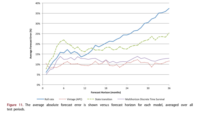
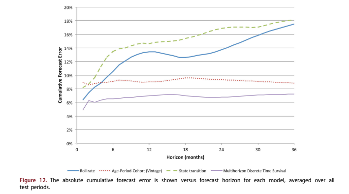
Figure 11 shows the median average absolute error across tests by forecast horizon. Figure 12 shows the cumulative forecast error with fore- cast horizon.

For the first three months of the forecast, the roll rate, state transition, and multihorizon DTS models outperform the vintage model. This is consistent with industry observations. Since roll rate and state transition models focus on delinquency and the results above show the importance of delinquency, this is to be expected. The vintage model does not consider any current performance information, so it is prone to near-term discontinuities.

However, in the long-term, the vintage model largely maintains its level of accuracy due to its emphasis on the lifecycle effect. The roll rate and state transition models deteriorate substantially over the long-term, because delinquency loses its predictive value. Since both models are one step ahead predic- tors, their coefficients are optimised for the near-term use of delinquency and largely lose sensitivity to other possible effects that would be useful in long-term forecasting.

The multihorizon survival model outperforms all models in the early months and attains a long-run accuracy just above that of the vintage model. When the cumulative errors are considered, the early advantages of including delinquency give the multi- horizon survival model an advantage over the vin- tage model.

7. Conclusions

The multihorizon survival model achieves its intended goal of being more accurate than other models for short term forecasting and comparable to vintage models for long term forecasting. Many organisations currently use two separate models for short-term and long-term forecasting, so this pro- vides a best-of-both-worlds approach in a single modelling framework. This is particularly beneficial in the context of IFRS 9 and CECL so that accurate loss reserves are created that capture the best cur- rent information about the loans and the lifetime expectations.

In the process of estimating the multihorizon sur- vival model, reviewing the coefficients versus fore- cast horizon appears to explain this performance advantage. For short horizons, the coefficients cap- ture the extreme nonlinearity of delinquency. For longer horizons, these coefficients capture the rate of decay of information content across explanatory variables, generally replacing short term predictors (delinquency) with long term predictors (LTV, DTI, etc.).

Although originally designed to solve the lifetime loss forecasting problem for IFRS 9 and CECL, this modelling technique provides advantages in many other contexts. As a behaviour score for account management or collections, the forecasts can be aggregated over any desired horizon. Given an eco- nomic scenario, the” score” is immediately cali- brated to a probability. Moving from rank-order scores to probability estimates has immediate advan- tages across a range of applications, such as loan pricing and cash flow estimates for existing loans.