Normalizing Pandemic Data for Credit Scoring

Abstract

The COVID-19 pandemic created abnormal credit risk conditions that did not align well with pre-2020 credit scores. Since the pandemic, most organizations have either excluded the period 2020-2021 from their modeling or included it without adjustment, leaving it as noise in the data. Model validators and examiners have been divided about requiring one of these approaches or defaulting to model developer judgment. None of this is ideal from a model development perspective. We have found that a technical solution is available. Our analysis uses lifecycle and environment outputs from an Age-Period-Cohort analysis as fixed offsets to the credit score development. Panel data is used, so the credit score is developed with a discrete time survival model approach. We tested logistic regression and stochastic gradient boosted regression trees as estimators with the panel data and APC

inputs.

For this research, we used Fannie Mae data. The APC model was estimated on the full available history, from 2005 through 2024. The origination scores were estimated on two-year periods from 2016 through 2024 and tested on all other periods, including a score that was developed on the full period. All models were also tested on comparably prepared data from Freddie Mac for cross-validation.

1. Introduction

The COVID-19 pandemic created unprecedented economic conditions that fundamentally disrupted traditional credit risk assessment. According to research on marketplace lending, the probability of loan default increased from 0.056 in the pre-pandemic period to 0.079 during the pandemic. This significant shift occurred despite massive government intervention programs designed to stabilize the economy [6].

These intervention programs, while beneficial for short-term economic stability, created additional challenges for credit risk assessment. A study by [3] found that default intensities shifted from long-range to short-range dependence during the COVID-19 period, making historical credit perfor- mance much less relevant for credit prediction. This phenomenon contrasts sharply with previous financial crises, where long-memory patterns remained relatively stable. The current research appears to present a solution to this challenge.

Financial institutions faced significant challenges in implementing credit risk models during this period. The disconnect between economic condi- tions and credit performance led many institutions to replace advanced credit scores with simple bureau score-based decision trees.

Traditional credit scoring models faced particular challenges during the pandemic for several reasons. The rapid implementation of forbearance pro- grams artificially suppressed delinquencies, creating a disconnect between observed credit performance and actual credit risk. Consumer spending patterns changed dramatically as lockdowns limited discretionary spending opportunities, leading to decreased credit utilization and paradoxically im- proved credit scores during a period of economic distress. This created what Breeden [8] termed “Macroeconomic Adverse Selection”, where the macroe- conomic environment significantly influenced the distribution of consumers applying for loans in ways not reflected in their credit scores. The impact of the pandemic was heterogeneous across different segments of borrowers, with certain industries and geographic regions experiencing more severe ef- fects [30].

A fundamental limitation of traditional credit scoring approaches is their reliance on cross-sectional data rather than panel data. Cross-sectional mod- els provide only a snapshot at a single point in time, failing to capture the dynamic nature of credit risk as it changes through a loan’s lifecycle and across different economic environments.

Panel data approaches, which track the same borrowers over multiple time periods, offer several advantages for credit risk modeling [36]. By knowing when a loan defaults, the model can be designed to distinguish between defaults that occur due to the maturing of the loan, shifts in the economic environment, or the intrinsic credit risk of the loan. During economic shocks like the pandemic, these advantages become even more critical as they allow models to adapt to changing conditions and capture time-varying effects that cross-sectional approaches cannot address.

This paper introduces a method to normalize pandemic data for use in credit scoring. The lifecycle and environment functions from an Age-Period- Cohort (APC) model are used to normalize panel-structured performance data. With this normalization, logistic regression and stochastic gradient boosted trees are created on Fannie Mae and Freddie Mac mortgage data to create origination scores that maintain predictive power despite the pan- demic’s unprecedented conditions.

2. Model Architecture

Many lending analysts have tried to create macroeconomic indices to measure the actual impact of the pandemic on consumers [16, 21, 20, 29]. The author tried creating an index of “persons receiving income”, which would include employed people and those receiving government support. Although this and other indices made sense, none could capture the impacts of the various forbearance programs and benefits. Rather than a macroeconomic-based approach to normalization, the most effective method was to measure the net impact via age-period cohort modeling and then adjust the score estimation to use the observed environmental impacts for normalization.

    2.1 Fundamentals of APC Modeling

Age-Period-Cohort (APC) analysis provides an effective framework for mod- eling default risk over time [38, 26]. Originally developed in epidemiology and sociology [28], APC models have been used in loss forecasting and stress testing [7]. These models decompose credit performance into three funda- mental components: lifecycle effects versus age of the account, environmental impacts versus calendar date, and credit quality by vintage.

The basic APC model can be expressed as

log-oddsPD(a, t, v) = F (a) + G(v) + H(t)    (1)

PD is defined in this context as Ever 60+ DPD Rate, meaning a ”default” is recorded on the first occurrence of an account becoming 60 or more days past due. a is the age of the loan, t is the calendar time, v is the vintage date, F (a) represents the lifecycle function, H(t) represents the environment function, and G(v) represents the vintage quality function.

This decomposition allows researchers to separate the effects of vintage quality from loan aging and macroeconomic conditions. During economic shocks like the COVID-19 pandemic, the environment function captures the impact of changing consumer financial conditions, while the vintage function reflects changes in borrower quality. The ability to measure actual impacts via H(t), rather than trying to explain calendar date impacts purely from macroeconomic factors, was a key to success during the pandemic.

One challenge in APC modeling is the identification problem arising from the linear relationship a = t−v [27]. Various approaches have been proposed to address this issue, including imposing constraints on the functions. In credit risk applications, a common approach is to represent the model as

log(PD(a, t, v)) = b0 + b1a + b2v + F ′(a) + G′(v) + H′(t)    (2)

where F ′(a), G′(v), and H′(t) are nonlinear functions with zero mean and no linear component. This formulation resolves the linear trend ambiguity. The analyst must then decide how best to allocate the trend, considering the details of the problem. For the analysis here, the environment function is chosen to have zero trend, which is most appropriate with long time histories spanning more than one recession. If less than one economic cycle had been available, fitting to economic factors while allowing for a secular trend can resolve the environmental trend uncertainty.

The functions are estimated using a Bayesian Age-Period-Cohort algo- rithm [32], in order to constrain the estimates for recent vintages and older dates where few observations are available.

    2.2 Panel Logistic Regression with APC Inputs

Many credit scoring techniques exist which leverage survival modeling prin- ciples [22, 34, 33, 5]. The most common of these is Cox proportional hazards

[18, 35, 31], which is widely used, but suffers from instability in a credit scoring applications [11].

To implement discrete time survival models with APC inputs, we use panel logistic regression with an augmented model matrix [14]. One row is created per account per month active, and no more than one entry for a default event. Censoring the data after default means implicitly that the de- nominator for PD will be the previous month’s open accounts. This structure allows the analyst to include a parallel model of the probability of prepay- ment in order to consider competing risks.

The model matrix becomes

where the first column is the default indicator, the second column is the life- cycle at each age, the third column is the environment function at each time, and the remaining columns are scoring covariates. During model estimation, the coefficients for the lifecycle and environment columns are fixed at 1.0.

By including the APC lifecycle and environment functions as fixed inputs, the panel logistic regression model can be expressed as:

where sij are the available attributes at origination for account i, and the cj are the coefficients to be estimated. This approach allows F (a) + H(t) to specify the mean of the distribution at each forecast month, with the logistic regression model estimating the distribution of account risk centered about that mean. In other words, the credit score models the residual risk after adjusting for lifecycle and environment, thus normalizing the performance data for account age and the pandemic conditions.

This approach significantly improves out-of-time performance compared to traditional credit scoring methods [14]. By providing lifecycle and envi- ronment functions as fixed inputs to the model, we can achieve more stable coefficients for risk factors and better capture the impact of changing eco- nomic conditions.

    2.3 Stochastic Gradient Boosted Trees

Machine learning methods, particularly gradient boosted trees, have gained popularity in credit scoring due to their ability to capture complex, non- linear relationships in data. Stochastic Gradient Boosted Regression Trees (SGBT) combines bagging with gradient boosting to create an ensemble of ensembles of trees [19, 25].

The basic idea of gradient boosting is to build subsequent models on the residuals of previous models, computing the gradient of a fitness function to provide weights to each model trained. Stochastic gradient boosting adds randomization to this process, building different gradient boosted ensembles for each data subsample.

where each hk(x) is a model and ν is a learning rate parameter. This approach can significantly reduce computation times while maintaining acceptable ac- curacy.

When regression models are used for the hk(x), then lifecycle and envi- ronment may be included as fixed offsets, just as was done for the discrete time survival model [14]. The input data is again structured as a panel, so the resulting forecasts are monthly, conditional PD. Other researchers have developed combinations of survival modeling and stochastic gradient boosted trees [17, 4, 37, 1, 2], although for the current problem, we prefer the APC approach of incorporating an empirical environment function for normalization of the creditt score development.

3. Fannie Mae and Freddie Mac Data for Orig- ination Scores

To demonstrate the approach, loan-level data from Fannie Mae and Freddie Mac were analyzed. The Freddie Mac Single Family Loan-Level Dataset covers approximately 53.8 million mortgages originated between January 1, 1999, and June 30, 2024, with monthly loan performance data through September 30, 2024 [24]. Comparable data from the Fannie Mae Single- Family Loan Performance Data was prepared for modeling [23]:

For our analysis, we focus on loans with FICO scores between 660 and 780, following the approach described in the search results. This creates a dataset with 622,452 unique loans of which 4,346 defaulted for a lifetime default rate of 0.7%. The data includes vintages from January 1999 through November 2019, with performance data from January 2017 through December 2019.

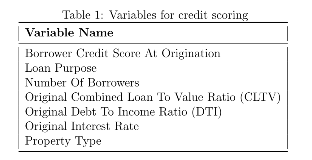
The origination scoring variables available from both Fannie Mae and Freddie Mac are given in Table 1.

This set of variables is sufficient to demonstrate the approach, but not to highlight the nonlinear modeling capabilities of the stochastic gradient boosted regression trees.

To prepare the data for our panel modeling approach, we create an aug- mented data matrix where each loan has multiple observations corresponding to different points in its lifecycle. For each observation, we include both static variables (such as bureau credit score and LTV at origination) and the values of the APC functions.

4. Results

    4.1 Age-Period-Cohort Model

For the APC analysis, the full Fannie Mae data was analyzed. This was necessary in order to estimate the environment function over the full date range. For all in-sample and out-of-sample test results, the actual environ- ment function was used. This means that out-of-sample or out-of-time refers

to the data used for training the score. This approach is called an ”ideal sce- nario validation”, because we do not want to confuse our scoring model tests with errors from predicting the environment function using macroeconomic variables.

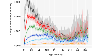
The environment function clearly shows the 2001 and 2009 recessions and the 2020 pandemic, Figure 2. The lifecycle functions, Figure 1, mirror those observed previously [9].

The APC vintage functions, Figure 3, clearly show the strong periods of adverse selection from 2006 through 2008 [12] and more recently from 2022 through 2024 [10]. These periods have previously been explained as arising from sudden shifts in interest rates, causing a shift in the intrinsic risk of the loan applicants in ways not visible from standard scoring attributes. This effect was also observed in auto loans [13] and other consumer loans [15].

For purposes of demonstrating normalizing pandemic data for scoring, the vintage function was not included in the credit score, and macroeco- nomic adverse selection was not estimated after score construction. If these models were put into production, researchers should continuously track vin- tage residuals and include these in the forecast in order to align the credit score forecasts from different periods. Vintage residuals are not exactly the same as the APC vintage function. Conceptually, they are equivalent to subtracting the credit score aggregated by vintage from the vintage function.

    4.2 Credit Scores

To test the credit scoring approach, models were estimated on two-year pe- riods and tested on all other two-year periods. For each type of credit score, this process created four separate models plus a fifth model spanning the entire range.

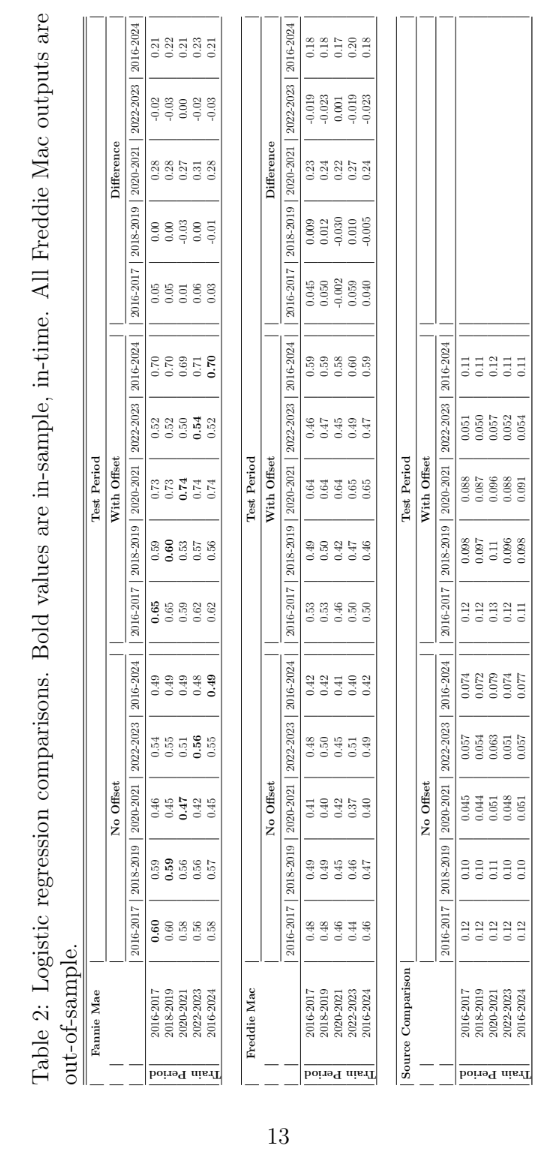
A panel logistic regression model was created with lifecycle and environ- ment as fixed offsets, as discussed earlier. All of the scoring variables from Table 1 were significant and retained in all models. Table 2 shows the Gini coefficients for each model. In-sample test values are shown in bold. Out-of- time test values are shown in regular type. The table is designed to facilitate the comparison of panel logistic regression models with and without the APC offsets. As shown in the Difference section, the difference is insignificant ex- cept for the period 2020-2021, in which case the model with an offset had a Gini coefficient on average 0.28 higher than the panel regression without a coefficient. The model built on the entire span had a comparable gain,

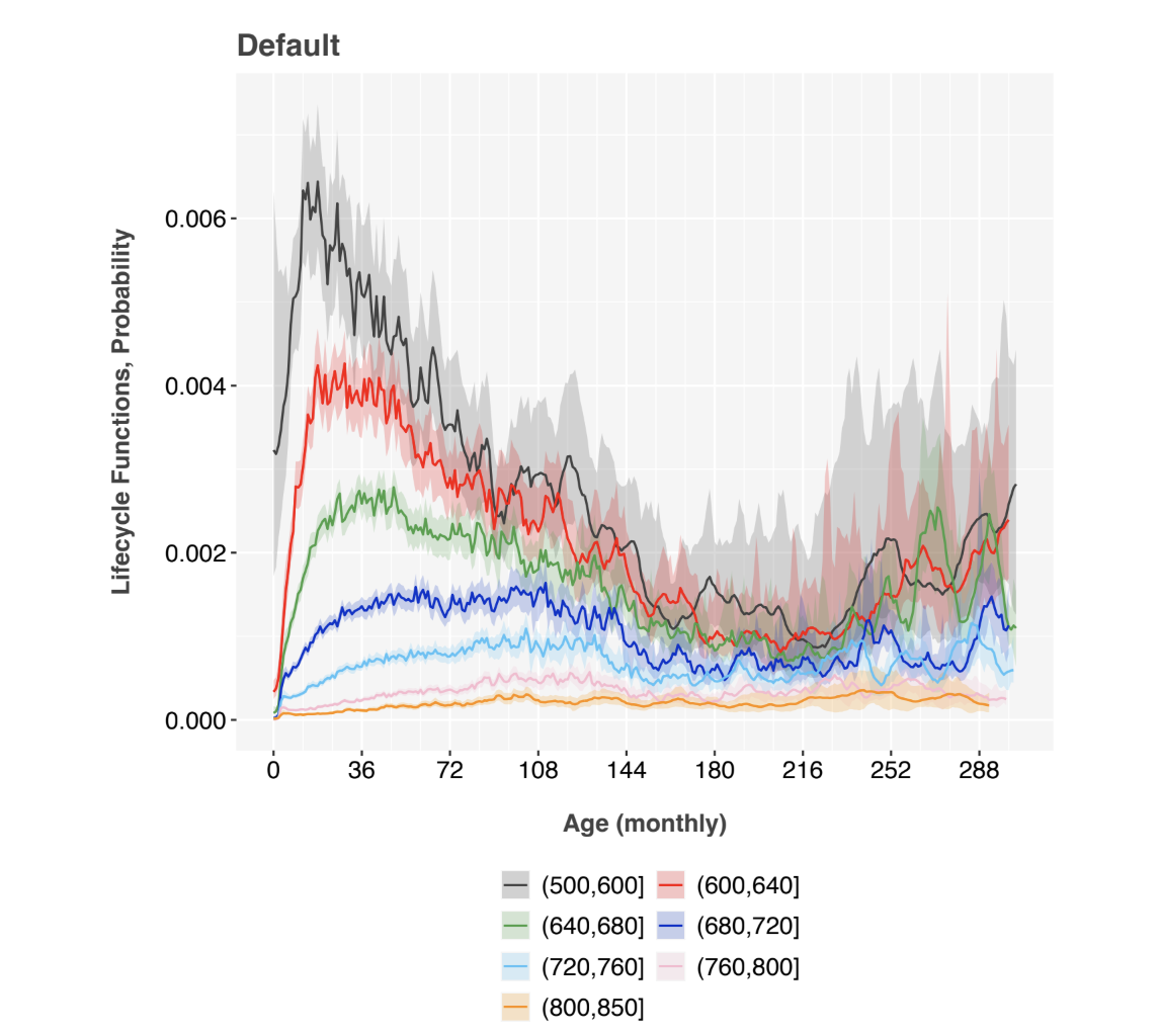
Figure 1: APC lifecycles obtained from Fannie Mae data, segmented by bureau score bands. The y-axis is in units of monthly probability of default.

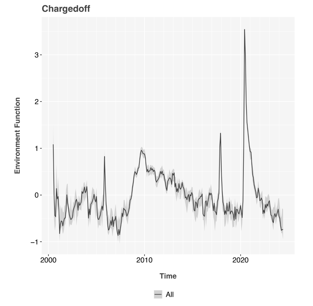
Figure 2: APC environment function for Fannie Mae data. Testing showed that the function was equivalent across segments considering confidence in- tervals. Therefore, a single overall function was used in later analysis. The y-axis is in units of log-odds of default.

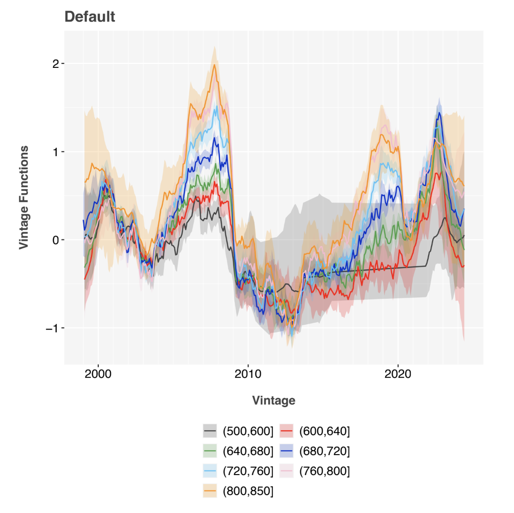
Figure 3: APC vintage functions, segmented by score band. The y-axis is in units of log-odds of default, so higher values correspond to riskier vintages even after segmenting by bureau score.

presumably because of the inclusion of the 2020-2021 period.

The section for Freddie Mac was included as a fully out-of-sample test, since none of this data was included in the model. The comparison of Freddie Mac to Fannie Mae could give an idea as to how much a score would degrade if built on Fannie Mae data and then applied to a lender’s in-house loan origination. The Freddie Mac results generally show a reduction in Gini of

0.08 relative to Fannie Mae, but with the same pattern regarding the 2020- 2021 period.

For the second test, a panel stochastic gradient boosted regression tree (SGBRT) was created. The SGBRT models were estimated on 60% of the in-sample data with 40% as a cross-validation hold-out sample. The meta- parameters for the SGBRT algorithm (number of leaves, tree depth, learning rate, number of trees) were optimized in-sample on the 2016-2017 time slice and used throughout. One model was given APC lifecycle and environment as fixed offsets, and the other was not. Those results are shown in Table 3 with the same format as for the panel logistic regression outputs.

The panel SGBRT models show slightly better performance than panel logistic regression in all tests, but the difference is not significant. The pattern across test periods is again the same as for Table 2, with the 2020-2021 period showing the greatest when including the APC inputs. The Freddie Mac out- of-sample testing was even closer to the Fannie Mae results.

Previous studies have shown improvement when using APC inputs, in- sample and most notably out-of-sample. The mortgage data is different, be- cause it is a very large data set with a wide range of vintages. When modeled over a short, two-year time window in a calm economic period with a lim- ited set of available scoring variables, the advantages of APC inputs largely disappear. For smaller, more dynamic portfolios of shorter-term loans, the APC lifecycle will be an important contributor.

During very dynamic economic periods, as seen in 2020-2021, the APC environment input is essential to creating an effective model. Perhaps iron- ically, the model built during this time period with APC inputs performs better in all time periods than the models built in-sample on those other time periods. This is likely due to the increased ability to separate envi- ronmental effects from scoring attribute dynamics when the environment is dynamic and clearly identified.

The lack of significant improvement from SGBRT as compared to LR is not a surprise. Much has been written trying to determine which model- ing algorithm is best without paying sufficient attention to the data being

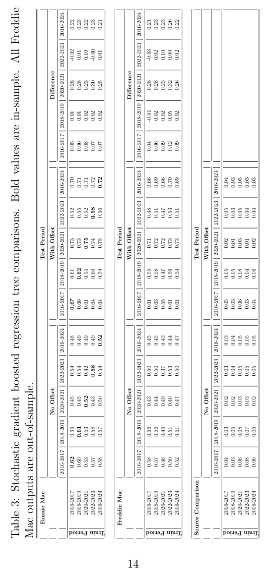
modeled. This mortgage data, where the scoring attributes are either lin- earized or predefined discrete factor levels, eliminates the need for SGBRT’s nonlinear flexibility.

Overall, our results confirm that incorporating APC inputs into both panel logistic regression and stochastic gradient boosted regression trees sig- nificantly improves model performance during economic transitions, partic- ularly the unprecedented conditions of the COVID-19 pandemic. This ap- proach not only allowed for the inclusion of pandemic data in the modeling but actually improved the resulting scores compared to excluding that data.

5. Conclusion

The fragility of credit scores to economic changes has often been accepted as unavoidable. This paper demonstrates that credit scores can be designed to be resilient through economic volatility and, in fact, benefit from volatil- ity. The keys to this resilience are 1) using panel data (one observation per account per month) rather than cross-sectional data (one observation per account for the full training window), and 2) integrating Age-Period- Cohort lifecycle and environment into the credit score estimation, whether traditional logistic regression or machine learning.

This approach was quite effective for being able to model data from the worst economic period of the COVID-19 pandemic. One particularly power- ful aspect is that no macroeconomic variables were used. The pandemic is notorious for breaking the traditional correlations between macroeconomic factors and loan defaults due to the unprecedented government intervention and forbearance programs. The APC environment function can quantify what the environment was during any given time period without needing to explain what caused that environment in macroeconomic terms.

Although the current research focused on modeling defaults, the same methods can be applied to other key metrics, most commonly prepayment, attrition, and recovery rates. Although survival models are designed to model terminal events, the APC approach applies to any variable. For products such as credit cards, this can include modeling purchase, payment, utilization, and revolving balance rates.

The work here was performed on Fannie Mae and Freddie Mac mortgage default data. Similar analysis for auto, credit card, and personal loans inter- nally at banks with proprietary data has shown even more dramatic benefits because of the smaller, more dynamic portfolios being modeled.

The specific combination of APC and credit scoring is one of a family of algorithms that could be employed to achieve similar goals. Broadly speak- ing, combining discrete time survival models and machine learning models can overcome many shortcomings of today’s credit scores.