A Theory of Borrowers

Introduction

Lenders have been creating credit scores for decades, and yet, every credit score is created as if it were the first time. We explore the data as if we do not already know the answer from those decades of prior experience. We attempt to estimate all of the needed coefficients from the small sample of data that we have. Machine learning is the worst at this, because we are encouraged to let the algorithm learn empirically from the data rather than being guided by the analyst. The data is dumped in, and the algorithm must learn everything from the beginning. Not only is this inefficient, but it leads to less effective models.
A purely data-driven approach can lead to odd outcomes. With a logistic regression approach where we can interpret the estimated coefficients, we can at least impose some constraints. Increasing bureau score must imply decreasing default risk, unless the originations team has done something terribly wrong. Increasing unemployment must lead to increasing defaults, unless something in the economy is fundamentally broken. If our data was predominantly from the COVID-19 pandemic, these relationships might not hold, but would we want to use a model that learned the opposite? Even though we understand now that unemployment and default rates went in opposite directions during the pandemic, that is not the model we would want to use going forward.
With machine learning, the world seems to be moving toward a data-driven approach on the assumption that the “big data” being gathered knows more about the subject than industry experts do. We can make some convincing arguments that the opposite is true in lending, primarily because economic cycles and credit cycles can span a decade, whereas today’s “big datasets” seldom extend more than a few years. This leads to a fundamental confusion between economic cycles and intrinsic borrower risk, which is a leading cause of out-of-time degradation of machine learning models.1
Not only will machine learning models get confused between slices of long cycles and intrinsic consumer behaviour, they can only predict based upon the factors they have. Anything that is not an observed input is left to the unexplained residual. These residuals have not been studied as carefully as they should have been. Simply looking at credit score residuals by vintage reveals fascinating structure, which has led to a better understanding of macroeconomic adverse selection.2
The current paper is a deeper philosophical exploration of what lurks in that unexplained residual of borrower behaviour. Can we see deeper into adverse selection and what dimensions of borrower behaviour are completely invisible to us when we see only credit bureau data?

Background

Economists have developed many theories of consumers and consumer choice. Classical economic theories that treat consumers as financially rational decisionmakers are not well supported by what we see in lending data. Basic marketing principles appear to belie the rational consumer hypothesis. Instead, the field of behavioural economics comes closer to lenders’ experiences. For example, hyperbolic discounting3
is a behavioural economic theory describing how people tend to prefer smaller, immediate rewards over larger, delayed rewards, and how this preference changes over time in a non-linear way. This theory contrasts with the traditional economic concept of exponential (or rational) discounting, where the value of future rewards decreases at a consistent rate over time. Certain loan products could be viewed as leveraging the arbitrage opportunity between the hyperbolic discounting implicit in consumer preferences and the NPV calculations in finance. If we consider borrowing behavior specifically, Basel II4
is probably the best-known theory of behaviour. The model used for Basel II capital calculations can be viewed as starting from an assumption that defaults occur when the borrower’s debts exceed their assets. This is used to derive a one-factor model where external shocks could drive the borrower into default. This formula fails conceptually for several obvious reasons. First, it ignores predictable volatility. As the borrower matures through the life of a product, their risk of default changes, as quantified by survival analysis5,6,7 or Age-Period-Cohort modelling8
. When viewed as a portfolio, vintages reach peak risk levels at different times, so variation in loan volumes creates predictable volatility in default rates that should not be considered when computing capital. The Basel II formula precludes understanding risk versus the product lifecycle, which ironically has been seen to be one of the dominant factors. Further, the notion of defaulting when liabilities exceed assets may be true for companies, but bears little relationship to consumer behaviour. A consumer needs a home, so a fall in the market value of that home relative to the associated mortgage only matters for investment homes or new residences where the borrower has no established existence. Proximity to school, home, family, and friends provides utility value that is not easily measured but usually exceeds market fluctuations in home values. Similarly, older cars have little resale value, but are still necessary for sustaining one’s lifestyle. Uncollateralized loans are the most obvious example, where the utility value and reputation risk (via the credit bureau) are the determinants of default, rather than any assessment of assets and liabilities. In fact, some segments of the younger generations are moving more to a rental existence, bringing forward their spending in order to support a better lifestyle. Throughout their lives, they may never achieve positive net assets and yet they may default no more than current experience.

Some might argue that a theory of borrowers can already be created from what is known in classical and behavioural economics. It is true that much is known about consumer and corporate behaviour in the economics literature, although the interaction between a consumer
and a loan product creates specific risks for which lenders have better data than economists. An expanded treatise would be needed to do justice to the economic literature, but a few comparisons are worthwhile. For example, the differences between an individual outcome and the probabilistic distribution of outcomes for an individual are fascinating. Each of us has only one lifetime. The stock market might return 7% to 10% annually when measured over decades, but for a person whose peak earning years are during their 50s and who hopes to retire in their 60s, only one-decade matters. The realized return for that person could be quite different from the average. Humans are rightfully more risk averse than statistical algorithms suggest, and this insight is embedded through millions of years of evolution. Therefore, a recommendation algorithm for a single person must be designed to much more heavily weight the risk tails than would be true for a distribution of people observed over decades. This is a key insight of behavioural economics, called Prospect Theory9
, suggesting that people value gains and losses differently. It shows up in the Gambler’s Ruin, theories for optimal bet sizing, and almost any risk assessment done through a person’s lifetime. Insurance arises naturally to address this problem. A hundred years ago, a fire burning down a home could financially devastate a family for a generation. Fire insurance distributes this risk so that we can all share the cost as if we were living a distribution of lifetimes. Some insurance may be about distributing risks across my own lifetime, but the best societal use of insurance is to allow me to live as if I experienced a distribution of thousands of lifetimes. These principles appear in lending, in that some loan products provide the same opportunity for the consumer to live across a distribution of lifetimes, smoothing their spending over time with borrowing and repayment.
Whereas lenders help borrowers manage their distribution of possible lifetimes, regulators are managing a distribution of lenders, helping smooth the risks across the realized lifetimes of those lenders. A theory of lenders might be created that might share a lot in common with the theory of borrowers.

A Basic Framework

To be useful for modelling, a theory of borrowers needs to be equation based and incorporate as many aspects as possible. This means that the usual cross-sectional data credit scoring perspective is insufficient. Instead, we need to think about how borrower behaviour changes through the life of the product. We can think of this as a cash flow perspective on the borrower or a panel data perspective when analysing a single target variable. Discrete time survival models and age-period-cohort (APC) models provide a natural framework for thinking about borrower behaviour.
10 The data that we gather on loan performance is observable in three time dimensions (age of the account, calendar date, origination date), which also aligns well with the intrinsic drivers of behaviour. When modelling the log-odds of default, an APC model can be written as

logit(default) = lifecycle(age) + credit quality(vintage) + environment(date)

We cannot prove why these pieces must be separable. If we simultaneously model borrowers across a wide demographic range or consider multiple loan products, these pieces are not separable. However, if we do select a specific product for a specific demographic group, with sufficient data that we are not just dominated by low-event-rate noise, the APC framework routinely explains 99% of the structure of the data. It is as if we performed a principal components analysis (PCA) and found that the first three vectors have intuitive explanations and capture almost all of the structure. It’s an empirical result, but one supported when looking across twenty years of Fannie Mae and Freddie Mac mortgage data, and in-house data from all other loan types.

Lifecycles

Understanding the lifecycle versus the age of the loan is an essential starting point. Fortunately, it is also the most universal. The shape of the lifecycle is specific to how a demographic segment interacts with a specific loan product, but universal across lenders and often across countries. This means that the way consumers use loan products is innate to our societies and personal finances.
At the point of underwriting, the lender does their best to make sure that the borrower can repay the loan. However, a subprime borrower is someone who has shown difficulties paying their debts in the past. The lifecycle for subprime mortgage borrowers shows that the risk of default for these borrowers rises rapidly through the first several years before reaching a saturation level around the fourth year. Conversely, superprime borrowers show rising risk throughout the life of the loan, because the most financially capable borrowers are the most likely to prepay or refinance their loans. The original pool of borrowers becomes ever riskier because of this selection bias. Since subprime borrowers are unlikely to be able to prepay or refinance their loans, the risk in the surviving pool reaches a constant level.
This explanation of the lifecycles could be written with a specific functional form, but it does not prove the hypothesis just put forward. Other aspects also affect lifecycles, such as rate resets, end of term, the end of introductory rate periods, and balance transfers. A library of such curves can be created, because of their universality. A new borrower can be assigned to a lifecycle, even for a new product with limited history, as long as the product matches a known type. In other words, this demonstrates that most loan products are standardized commodities. When analysing US mortgage data, we can easily show that the shapes of the lifecycles have not changed in decades.
The lifecycle variation observed by segment suggests that we could have a lifecycle surface across dimensions of age and demographic risk, perhaps measured by a bureau score. Although true, measuring such a surface nonparametrically from loan performance data in an enhanced APC approach has proven to be difficult. I have not yet identified a functional form that can be morphed to match each of the lifecycles within such a library.
Although lifecycles can be quite complex for certain product segments, commercial loan lifecycles are clearly much simpler than consumer loan lifecycles. Whereas consumers assign personal utility to a loan product in complex ways, commercial borrower lifecycles tend to look like the prime mortgage lifecycle. This appears to be due to the borrowers being companies with sufficient financial expertise that borrowing and default decisions are comparatively unemotional. Companies are closer to the rational consumers of classical economics. Small business borrowers are a mixture of the two.

Environmental Impacts

If we determine the lifecycles empirically and also accept empirically that these effects are additive, then the next piece to consider is the environment versus calendar date. The additive structure means that economic shocks affect all borrowers proportionally, regardless of the age of the loan. Within a product segment, this is a surprisingly accurate assumption, but it did not need to be this way. One could assume that new borrowers are more sensitive than seasoned borrowers, however, the proportional assumption holds true.
The environment function is usually thought of as exogenous impacts on the borrower. This can include the economy, seasonal effects, changes in laws and regulations, government policies, lender policies, natural disasters, and anything that impacts all borrowers in a portfolio on a specific calendar date. Too often analysts will try to include macroeconomic measures in their models without first measuring the net impacts. An APC analysis quantifies these impacts like a seismograph trace. The analyst can then look for how best to explain it.
Macroeconomic variables usually are the best way to explain the long-term patterns in the environment function. This modeling should not be performed as a search across all available macroeconomic factors, because we never have enough economic cycles to create a completely empirical model. Instead, we start by knowing that the correct answer will include some combination of the unemployment rate, change in GDP, change in house prices as the largest asset of home owners, change in interest rates for prepayment rate modelling, and a small set of other candidate variables specific to various loan types.
The hierarchy of payments is reflected in the sensitivity of the environment function to macroeconomic factors when comparing across products. The economy will impact borrower defaults on all products, but those most important to the borrower will show defaults slowly and with less sensitivity to external shocks.
Interestingly, from an individual borrower’s perspective, all that matters is whether they are still receiving income to support their normal expenses. Real disposable income is often considered as an aggregate measure of the consumer’s financial position, but this is rarely available segmented by the demographic groups as we would like, nor does it include everything that affects the borrower’s finances, for example changes in taxes.

The Dimensions of a Borrower

Within an APC framework, vintage risk is the aggregate credit risk of the borrowers within a pool. From the perspective of a single borrower, the APC lifecycle measures when they are most likely to experience difficulties with a product, and the environment measures the shocks to which the borrower is subjected. Borrower-level credit risk should assess the intrinsic risk of the borrower separate from the predictable lifecycle of the product and the impacts of the environment, primarily the economy.
Although a credit risk model can immediately be estimated in a discrete time survival model structure, inserting all of the available scoring factors with the known lifecycle and environment as fixed inputs, we should pause a moment to consider the primary dimensions along which we can understand borrower behaviour.

Lessons from Adverse Selection

For any credit risk model that has been previously built, forecast error can be measured by vintage. This might be done by creating a logistic regression model with the original score in units of log-odds as a fixed input and a set of vintage dummies. For all the models we have tested, the error by vintage is strongly auto-correlated. Durbin-Watson or Ljung-Box11 tests will immediately flag such models as being incomplete, yet scores are rarely tested this way, so model developers are rarely aware of this dramatic structure gap. Obviously, our models are missing something.
A small literature exists on adverse selection that explores these model residuals. The original version of adverse selection is that if a lender offers loan prices that are noticeably worse than competing lenders, the better borrowers will go to those competitors, and the overpriced lender will be left with excessively risky loans.12 The key point here is that the score could not see this. Bureau data and bureau scores summarize past performance. They do not distinguish between being lucky and being thoughtful, or being unlucky and being irresponsible. Lenders rarely have hard data to confirm the cause of adverse selection, because they cannot see the better accounts who applied elsewhere.
Macroeconomic adverse selection has more recently been identified by noticing that the residual risk from credit scores can correlate to changes in economic conditions.13 Most compelling is that these residual risks are synchronous across the industry and not idiosyncratic to specific lenders. The most obvious drivers of macroeconomic adverse selection are changes in interest rates and changes in the cost of the home or auto being purchased. That leads to the hypothesis that some borrowing pools are higher risk, because the value shoppers have pulled out of the market. “Value shopper” is a personality trait not identifiable from standard bureau data bureau data, so this makes a case for hidden variables or entire dimensions of borrower behavior that are invisible to our models.

Finding the Hidden Variables

Adverse selection is an aggregate measure that proves something important is missing from our models. By tracking model residual risk by vintage, lenders can get an early warning that borrower pools have changed, not all borrowers are risky. And during times of low residual risk, not all borrowers are low risk. Can we develop new data sources and metrics to reveal these dimensions beyond the bureau scores?
Several research groups have been exploring the use of alternate data to create borrower personality profiles. Credit risk assessment14 has been performed using the Big Five (BF) Model of Personality15: Extraversion, Agreeableness, Conscientiousness, Neuroticism, Openness and the Myers Briggs16,17 frameworks. Although they assert that these methods can be effective, we may have a problem with regulators. US law prohibits lending that disadvantages protected demographic classes. In response, lenders try to make sure that their lending decisions are not correlated with the dimensions of protected classes. Personality profiles are not among the protected classes, wider adoption might create a negative consumer response.
Rather than trying to know everything about a consumer, can we focus on just the dimensions relevant to lending and try to do so in non-intrusive ways? No such borrower personality framework currently exists, but a decade of studying residual risk by borrower pool has led me to propose the following as a conceptual framework that focuses only on borrowing personality traits and may be testable with some data sets available today.

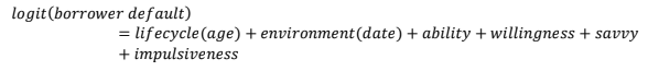
A Borrower Personality Framework

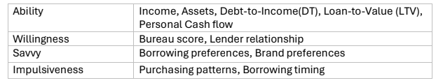
The lifecycle and environment are intuitively clear. Developing a theory of the borrower is understanding the key factors that determine the borrower’s credit risk after removing the lifecycle and environmental effects. I suggest the following categories to explain the borrower’s intrinsic credit risk.

1. Ability to pay
2. Willingness to pay
3. Financial savvy
4. Impulsiveness

The borrower’s ability and willingness to pay are the conceptual foundations of today’s credit risk models. Ability to pay refers to whether the borrower has sufficient income, stable employment, assets and savings, and manageable levels of debt and other financial obligations. The Debt-to-Income ratio is a standard part of a lender’s credit score. Some of these items are part of the verification process.
Willingness to pay is the domain of credit bureaus. Does the borrower have a demonstrated history of paying their bills on time? This is distilled into a bureau score, although the bureau score may be incorporating past misfortunes as much as willingness. In addition, does the borrower have an established relationship with the lender so that they are more inclined to trust and work with the lender should they encounter financial difficulties.
Financial savvy is demonstrated by what financial products the consumer avoids. Some products are not the best use of a consumer’s financial resources. A credit bureau scan showing certain loan products could be a risk indicator, although it is usually the nuances not reported to the bureaus that are most telling. Getting a loan for a new truck can be a necessary, well-reasoned decision. Getting that truck with overpriced trim packages that add little practical value could be a credit risk indicator suggesting a lack of financial savvy. We have recently seen a dramatic expansion in consumer loan products. Buy-now-pay-later options at checkout for online stores, travel financing, and payday loans appeal to very different levels of financial savvy. For example, cash loans appear riskier than purpose-driven loans. A consumer’s preferences in different interest rate environments can speak to financial savvy. At higher interest rates, moving to a longer-term loan in order to manage payments can be sensible, with an intention to refinance to a lower rate in the future. Ultimately, financial savvy is a personality trait that could be quantified similarly to a bureau score.
Impulsiveness is the essential personality trait underlying our analysis of macroeconomic adverse selection. We would like to distil the personality profile to a single scale for impulsiveness, the spectrum between value shoppers and impulse buyers. Someone is unlikely to be a value shopper if they get a new auto loan or mortgage as prices and interest rates are rising rapidly, but interest rate cycles that can reveal this behavior may occur only once per decade. Instead, can we analyze the way people shop on a daily basis to quantify impulsiveness? This is a new area of research, but credit card purchasing patterns suggest that it may be possible.

So, to collect these thoughts, quantifying the intrinsic risk of a borrower could be a series of measures on a log-odds scale.

intrinsic risk = ability + willingness + savvy + impulsiveness

Each of the components of intrinsic risk can be a model leveraging different data sources.

In the absence of data, the average level of financial savvy for borrowers of a specific product at a lender may be the overall risk scaling relative to a bureau score.
To predict the monthly probability of default, intrinsic risk for a borrower replaces the credit risk function by vintage in the APC structure.

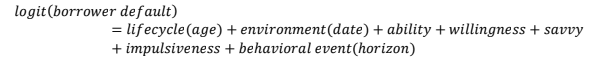
So far this looks like an origination score. What about behavioural data? Many of the measures on an individual account after origination represent a mixture of intrinsic and exogenous factors. The most familiar example is the borrower’s delinquency status. The borrower could be delinquent because they have financially risky personal habits, because of the impacts of a recession or natural disaster, because of unexpected personal tragedies including health care or divorce costs, or simply because this is the highest risk point in the product lifecycle for which the borrower was unprepared. Delinquency and other behavioural information should be thought of as shocks to the borrower, not necessarily a change to their intrinsic risk. To quantify the risk from the immediate shock, our models need to separate these effects in order to quantify how much incremental risk is evident from behavioural data, such as delinquency.
Over a short horizon, behavioural measures dominate the forecast as the borrower attempts to navigate their personal crisis. However, the information value of behavioural data dissipates rapidly as we create longer-term and lifetime forecasts. Therefore, behavioural data will appear as another term in our equation for the theory of borrowers with a dependence on forecast horizon because of the rapid dissipation rate for the information.
Alternate data does not fit into a single intrinsic risk category. Measuring savvy and impulsiveness will rely heavily on alternate data. Monitoring the borrower’s checking and savings accounts, with permission, is another kind of alternate data, specifically focused on identifying income and expense shocks. As such, this will be a leading indicator of delinquency and part of our measure of personal shocks.

In an ideal world, each of these components could be separately estimated. What we find in most credit scores is a mixture across components with missing pieces falling into the overall intercept or model residuals. Properly incorporating behavioral data requires a couple of steps in order to avoid double-counting with other components. Nevertheless, this can be done.
Having a logical framework is more than just useful for philosophical debates. Correctly assigning structure and incorporating available data reduces overfitting errors and long-range forecast biases, as observed in tests on incorporating APC inputs into machine learning models.
The lifecycle component is universal and may not change over decades, unless the product features change. The environment function is a measure of the current state of the world, so this is the dynamical component of the model. The borrower’s ability to pay will be dynamic and needs to be reassessed with each credit granting decision. Some lenders are experimenting with ways to educate borrowers about best practices in personal financial management, which may help with financial savvy. One assumes that this can improve naturally through the borrower’s lifetime.
The most intractable problems are willingness and impulsiveness. Bureau scores have been shown to be predictive over long periods of time, reinforcing the idea that willingness to pay may be innate. Similarly, impulsiveness may be a core personality trait that is unlikely to change. That makes estimating impulsiveness even more valuable as a lender manages their relationships with borrowers.
The above discussion tries to explain consumer behaviour, but some of this would seem not to apply to commercial loan borrowers. In fact, we have found that there are corporate analogues to all of the items described above. “Impulsiveness” might be viewed as “desperation” among commercial borrowers. When interest rates are rising rapidly, we observed a rapid rise in the credit risk of new commercial loan borrowers. After an extended period of low interest rates, which companies would borrow money at suddenly higher rates? Certainly not the usual borrowers. Financial savvy certainly can vary by company. The components of the theory of borrowers apply, just with different predictive variables.

Prepayment Behaviour

The discussion so far has focused on the reasons for default, which is our usual starting point. However, we also need to consider prepayment or attrition as part of our theory of borrowers. As with default modelling, we can begin the analysis with an APC decomposition, but the environment and vintage functions are not truly separable. The dominant factor in variations in prepayment rates for loans is the difference in loan interest rates available to the borrower at a future date compared to the rate the borrower obtained at origination. If we assume that APR is the rate available to the borrower assuming unchanged demographics, then APR(date) – APR(origination) measures how likely the borrower is to prepay.
Of course, available APR is not the only driver. Other economic conditions will have an impact, stressing the borrower’s ability to pay or the lender’s willingness to lend. Financial savvy will be a strong predictor of prepayment rates, as some borrowers simply pay more attention to the opportunities to refinance than others. Behavioural data will also be relevant, as delinquency and utilization will impact the borrower’s short-term ability to refinance.

The one factor that I am excluding from this formulation is “impulsiveness”. I have not seen clear evidence of model residuals from the above expression that would relate to personality traits of the borrower beyond financial savvy. Considering the importance of prepayment rates in assessing prime and superprime loan profitability, this warrants further exploration.
Attrition rates on lines of credit do not follow the same detailed dynamics as the prepayment rate formula. We might pay off a car loan or personal loan, but modern society is built around credit cards, at least until alternate payment mechanisms take over (PayPal, Venmo, Zelle, Alipay, WeChat Pay, Paytm, Boku, etc.). Therefore, consumers may move from one card to another based upon special offers, rewards, and credit limit. These are more about the product design and less about intrinsic borrower behaviors. Lenders often assume exponential decay as the base lifecycle for credit cards.

Conclusion

In a world with a rapidly expanding range of data sources, my primary goal in presenting a theory of borrowers is to encourage analysts to think about carefully about what each variable might mean. If we dump all of our data into a black box, we lose insights that could be used again. Alternate data to measure savvy or impulsiveness could be turned into scores for those attributes which the lender could use when considering a range of product offers to the consumer, just as bureau score is a transferable component to many decision models.
Although we have huge amounts of loan performance data, we never have enough through economic cycles, for new products, or for new data sources. The only way to build robust, effective models is to leverage our experience in order to design componentized models where different data sets are leveraged to estimate specific factors within an overall framework.
This approach also creates a better way to build machine learning models. For all of the same reasons, machine learning models will continue to be fragile unless we integrate the structure of what we know to be true. This is equivalent to assuming the framework described above and using machine learning models to estimate specific components within the framework. The final model will be a combination of APC components (lifecycle), macroeconomic sensitivity models, external scores, and machine learning models to estimate specific components (ability, willingness, savvy, or impulsiveness).
The final result is a set of models for decision making that are more accurate, more robust, integrate better into cash flow and yield models, and have greater interpretability and explainability.