CECL ASSESSING THE ALTERNATIVES

BY JOSEPH L. BREEDEN

A recent study used a large mortgage data set from Fannie Mae and Freddie Mac to test a range of models and options for implementing the Current Expected Credit Loss (CECL) method for determining the allow- ance for loan and lease losses.1 The results quantified the pros and cons of these options, all of which will be summarized in this article.

The Fannie Mae and Freddie Mac data provided origi- nation and performance information on conforming 30- year fixed-rate mortgages. In addition to monthly loan status, the database contained a number of attributes suitable for estimating loan-level credit risk.

Study Design

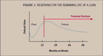
The biggest change under CECL will be moving to lifetime loss estimation. For an account of any age, the cumulative expected loss must be estimated for the remaining life of the loan, as shown in Figure 1. For example, with a 30-year term loan, the “lifetime” is simply 30 years—unless the loan pays off early. All forecasts must consider the competing risks of default and attrition (payoff).

Foreseeable Future

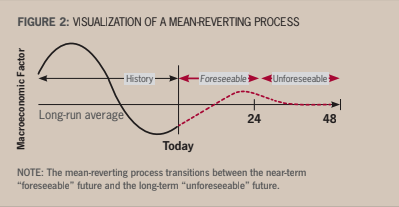
In all cases, scenarios were created with a 24-month macroeconomic history followed by mean reversion to long-run macroeconomic conditions. Many practitio- ners will likely create two separate models: a near-term model with a macroeconomic scenario and a long- run, through-the-cycle loss model. But using a single model with a mean-reverting macroeconomic scenario is preferable because the active portfolio is used for the lifetime loss forecast rather than an average of past portfolios. It also avoids the need to validate two separate models.

Twenty-four months was chosen as the “foreseeable” period in Figure 2, simply because this seems to be emerging as the standard for IFRS 9, which is further along in its adoption. One could argue that macroeco- nomic conditions are not foreseeable that far into the future. This will be yet another tuning parameter in CECL calculations.

Discounted Cash Flows

The guidelines also mention the option of using a discounted cash flow (DCF) approach. DCF is not a model so much as a system of equations for aggrega- tion, since it requires estimates of default and attrition probabilities as estimated in the models tested here. Therefore, all model results were created through direct loss aggregation, discounting of the monthly expected losses, and DCF aggregation of cash flows simulated from the loss estimation models.

Model Descriptions

The following models were tested be- cause they cover the range of options mentioned in the guidelines and are in common use. All models were created with segmentation in three risk grades: subprime, prime, and super prime. With- in those segments, all models were tested as a single U.S. national model and as 50 separate models by U.S. state.ƒ

Historical Averages

Averages of past history should not really be considered a modeling tech- nique. Historical average rates work only if everything is steady state: a constant economy, constant loan growth, and con- stant origination credit quality. In reality, none of these are true—which directly precipitated the call for CECL.

Moving averages are included here to provide a comparison of how loan loss reserves have most commonly been computed pre-CECL (not counting quali- tative adjustment factors), thus provid- ing a comparison between old and new practices.

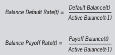
The averages were computed on the balance default rate and the balance pay- off rate so that all loans may be simulated through their remaining lifetimes.

Time Series

The simplest forward-looking model in this study requires creating macro- economic time-series models of the bal- ance default rate and pay-down rate. The rates are correlated to macroeconomic factors in order to create scenario-based forecasts. When these correlations were made, the macroeconomic factors were optimized for transformation (change, averages, etc.) and lagged effects.

by projecting these rates under a meanreverting base macroeconomic scenario until all currently outstanding balances are either paid off or defaulted.

Roll Rates

For the last 40 years, the two most common kinds of models for retail lend- ing portfolios have been credit scores and roll rates. Roll rate models are similar to a state transition model, but estimated on aggregate net balance flows from one delinquency bucket to the next.

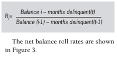
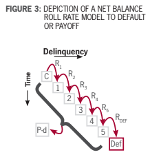
Each roll rate and pay-down rate are modeled as time series in the same way as the time-series model, using correlations to optimized macroeconomic factors to predict future values.

Vintage Models

Vintage models naturally capture the timing of losses and attrition versus age of the loan, and therefore they are an obvi- ous choice for lifetime loss calculations. Age-period-cohort models are commonly used to estimate such models.

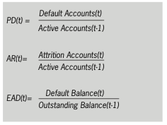
Because the models are applied to the account dynamics, the simplest set of key rates for modeling is probability of default (PD), attrition rate (AR), and exposure at default (EAD). Loss given default (LGD) is not being modeled. In- stead, recoveries are being held at 70% for all models.

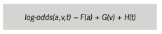
Each key rate is decomposed into a life cycle function versus the age of the loan F(a), a credit risk function versus origi- nation date (vintage) G(v), and an envi- ronment function versus calendar date H(v). The life cycle function captures the timing of losses or attrition. The environ- ment function is an index of sensitivity to macroeconomic changes, which is then correlated to macroeconomic factors as was done with the time-series and roll rate models.

The decomposition is performed as- suming a binomial distribution for PD and AR and a lognormal distribution for EAD.

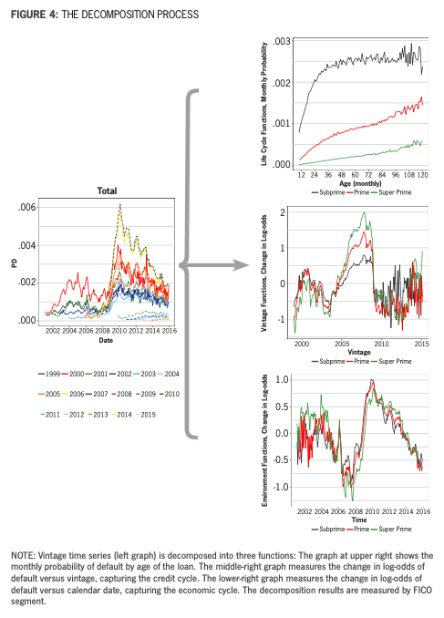
Figure 4 shows a visual example of the decomposition process for the subprime, prime, and super prime segments. The figure at left shows default rate time se- ries aggregated by annual vintage. The top-right graph is the life-cycle function transformed to the monthly probability of default, 1/1 + exp(-F(a)). The middle- right graph shows the change in log-odds of default by vintage, G(v), where the zero line is the average default rate. The vintage function shows the credit cycle with high-risk loans being originated in 2005 through 2008. The bottom-right graph measures the change in log-odds of default where the zero line is the aver- age environment, H(t). The environment function captures the economic cycle with the onset of the 2009 recession clearly visible.

Macroeconomic scenarios are used to project the future value of the environ- ment function, which is then combined with the vintage and life cycle functions to produce monthly forecasts for each vintage. Lifetime loss forecasts sum across vintages and calendar date to the end of the term or until the outstanding balance reaches zero.

State Transition Models

State transition models are the loan- level equivalent of roll rate models. They derive from Markov models, although in practice they may not satisfy the Markov criteria.

Rather than modeling aggregate move- ments between delinquency states, the probability of transition is computed for each account. The states considered are current, delinquent up to a maximum of six months, default, and payoff. Account transition probabilities are modeled rath- er than the dollar transitions in the roll rate model. Each transition rate model is actually a panel data model including multiple account attributes in order to predict the specific transition.

Discrete-Time Survival Models

Survival models are the loan-level version of vintage models with the inclusion of scoring attributes. Cox proportional hazards models are the original and classic approach to creating such models, but they were developed with continuous time in mind. For monthly sampled data such as is generally available in lending, discrete-time survival models are employed.

Once the change to discrete time is made, the result is just a logistic regression panel model of PD or AR. Practitioners commonly just include age as a factor in the regression, either non-parametrically or as a set of transformations as shown in the state transition model. Transformations of macroeconomic factors and scoring factors are included as well.

Separate origination and behavioral models are built, the former using only factors available at origination and the latter using both origination factors and behavioral factors such as recent delinquency. For the behavioral models, the coefficients are a function of forecast ho- rizon, because any delinquent account will have either cured or defaulted within six to 12 months. The remainder of the forecast is thus dominated by persistent factors like FICO score and loan-to-value.

Results

The following results are intended to be used for assessing trade-offs in CECL implementation details.

Accuracy

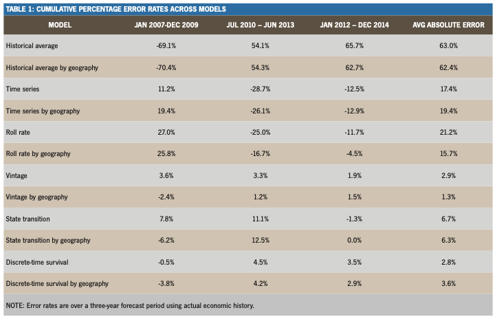
Projecting losses through time-series models of default and pay-down rates produced an average three-year cumu- lative error rate of 17% to 19%. In itself, that will raise concerns with validators, but the accuracy is unchanging relative to the amount of training data, which can be useful for very small or noisy data sets.

Vintage models were consistently high performers in terms of accuracy with error rates of 1% to 3%. Discrete-time survival models and state transition mod- els both performed well (3.2% to 6.5%), but not any better than vintage models, showing that loan-level modeling does not guarantee more accuracy. Vintage, state transition, and survival models all had similar scaling properties versus the size of training data.

Roll rate models were consistently the worst performers with error rates of 15% to 20%. Historical averages are unsuited to lifetime loss forecasting at 60+% er- ror rates. Overall, roll rate and historical average models should not be used for long-lived products.

Table 1 shows the cumulative percent- age error rates for all models.

Creating separate models by U.S. state did not provide greater accuracy when compared to a single national model of the same portfolio. Geographic segmen- tation provides advantages in business application but not model accuracy.ƒ

The guidelines indicate that vintage modeling is not a requirement. If we assume that “vintage model” refers to any approach that adjusts credit risk and prepayment risk based on the age of the loan, then the results show significant increases in accuracy for techniques in- corporating this (vintage models, state transition models, and discrete-time sur- vival models) compared to those that do not include it (time series and roll rate models).

Accuracy versus Complexity

The loan-level models (state transition and survival) were by far the most com- plex in terms of numbers of coefficients and computational time. This complexity did not provide any increased accuracy relative to vintage models, but it does pro- vide business value in account manage- ment, collections, pricing, and strategic planning.

The added complexity of roll rate mod- els compared to time-series models pro- vided little benefit other than the change to more accuracy for the first six months of the forecast. Vintage models were the overall winners in the trade-off between accuracy and complexity as long as suf- ficient data exists for robust estimation.

Lifetime Losses

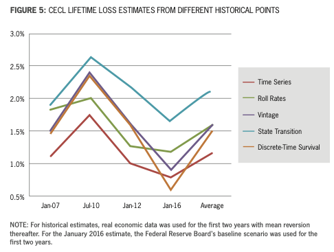
Figure 5 shows the lifetime loss esti- mates by model. Even though two models might show roughly equivalent results on the three-year accuracy tests, their ex- trapolation properties through the life of the loan could be quite different.

As shown in the graph, time-series models consistently had the lowest esti- mated lifetime losses, while state transi- tion models had the higher estimates with a 2x separation. This does not include historical averages (not shown), which were so high and volatile as to be off scale.

Time-series and roll rate models had very low volatility, presumably because they did not capture changes in the credit quality of loans. Vintage and age-period- cohort scores were the most volatile, probably because they were the most accurate in capturing the economic and credit cycles.

Optional DCF

If we start from a lifetime loss forecast, using a time-value-of-money discounting of the projected monthly losses with the effective interest rate on the mortgage results in a 20-30% decrease in the re- serve amount. Estimating the principal and interest payments adjusted for the risk of default or prepayment from the loss model, and then discounting with the effective interest rate, results in a 15-20% reduction in the loss reserves compared to the original lifetime loss forecast.

Old versus New Rules

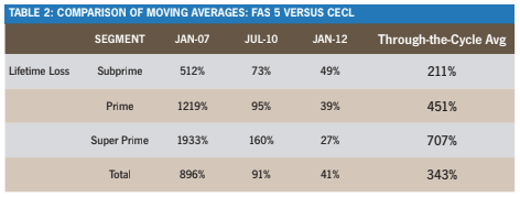
The magnitude of the change from the old rules in FAS 5 to the new rules of CECL will depend heavily on the lifetime of the asset and the point in the economic cycle when the adoption occurs. For 30-year fixed mortgages, the average life of the loan is about 5.5 years; thus, the lifetime loss reserve will be roughly four times higher than a historical average approach using a 24-month loss emergence period.

If adoption had occurred just before the onset of the last recession, the adjust- ment would have been 10x. At the peak of the recession, the change would have been 2x. Well into recovery, they would have been at parity.

Table 2 shows a comparison of a simple moving-average approach under FAS 5 with a 24-month loss emergence pe- riod and a lifetime loss calculation under CECL, using the vintage model with direct loss forecasts and discounted cash flows.

Conclusion

By design, the new CECL rules provide a significant amount of flexibility in imple- mentation. As seen from this study, even with a straightforward product like 30- year fixed-rate conforming mortgages, the range of models listed in the CECL guidelines can produce a range of lifetime loss numbers that vary by a factor of 2. With the option of discounted cash flows, the range of final results would vary by more than a factor of 2.

Being able to choose options that will create such different results will put the burden on lenders not only to choose the most appropriate models for their portfolios, but to defend that choice to validators, auditors, and examiners.