When Big Data Isn’t Enough: Solving the long-range forecasting problem in supervised learning

Joseph L. Breeden* and Eugenia Leonova

Prescient Models LLC, 1600 Lena St., Suite E3, Santa Fe, NM 87505, USA

Corresponding author

Abstract—In a world where big data is everywhere, no one has big data relative to the economic cycle. Data volume needs to be thought of along two dimensions. (1) How many accounts / transactions / data fields do we have? (2) How much time history do we have? Few, if any, big data sets include history covering one economic cycle (back to 2005) or two economic cycles (back to 1998). Therefore, unstructured learning algorithms will be unable to distinguish between long-term macroeconomic drivers and point-in-time variations across accounts or transactions. This is the colinearity problem that is well known in consumer lending. This paper presents a solution to the colinearity problem in the context of applying neural networks to modeling consumer behavior. An initial model is built using methods that are specifically tuned to capture long-term drivers of performance. That model is treated as given information to a neural network that then learns potentially highly non-linear dynamics relative to the given knowledge.

This approach of incorporating given knowledge into a supervised learning algorithm solves a deep but rarely recognized problem. In short, almost all models created via supervised learning will not give correct long-range forecasts when long-term drivers are present without corresponding data covering multiple cycles for those drivers. Thus, the need for such a solution is great and the solution provided here is sufficiently general that it can apply to a broad range of applications where both high frequency and low frequency drivers are present in the data.)

Keywords—forecasting; supervised learning; neural networks; data mining; age-period-cohort models

I. INTRODUCTION

Creating forecasting models for target variables that are impacted by both internal and external drivers is a well-known problem for statistical modeling. Examples of this include modeling consumer spending that is impacted by consumer behavior (internal) and economic factors (external) or credit risk modeling where delinquency (internal) and economic factors (external).

Since the internal and external factors can be correlated, properly separating effects is essential for accurate forecasting. Solving the problem is complicated when the external drivers have a short amount of data, such as economic factors. Learning algorithms have been very successful modeling large datasets when any cycles present are observed multiple times. However, in the case of economic data, the history is very short relative to the economic cycle, so mixing a short history for economics with a large data set for internally observed performance factors is a classic example of this problem.

This situation has previously been solved for regression-type models [2] In the specific context of creating loan-level stress test models of consumer loan delinquency, an Age-Period- Cohort model was used to capture two specific external drivers, economic impacts on delinquency versus calendar date and lifecycle impacts versus the age of the loan. This first stage modeling captures the long-term variation in consumer loan delinquency. The economic and lifecycle effects were then fed into a regression model as a fixed offset, meaning that their coefficients are each 1.0 in the final model. All other coefficients in the regression equation that are estimated on consumer behavioral attributes are estimated such that they provide adjustments relative to the fixed offsets but without changing those offsets. In this way, no problem arises from multicolinearity, because the offsets are taken as primary and the other coefficients capture the residuals.

In supervised learning generally, the training data contains observed values of a target variable and a set of candidate explanatory variables [8]. Supervised learning has been used previously for predicting time series such as economic time series [5,7] and separately for intrinsic behavior patterns such as credit scoring for offering consumer loans [10,1]. The problem just described in the context of regression models also applies more generally across supervised learning algorithms, where the same multicolinearity problem persists. However, many of those algorithms are unstructured and therefore lack the tools needed to solve the multicolinearity problem in a robust manner.

II. MODELING APPROACH

The present solution to the multicolinearity problem is a two- stage modeling approach. A first model is created that estimates future changes in long-term performance drivers. This could be an econometric model, survival model, or other types that capture long-term changes relative to calendar date or age of an account. This could more generally be treated as “given knowledge” obtained from models on other data sets or other sources. This given knowledge is treated as a fixed, known input to a second model, a supervised learning approach that may have much richer information to train on over a shorter time frame that what originally created the given knowledge.

If the target variable for the analysis is real-valued, then the solution is simple. The forecasts from the given knowledge are subtracted from the target variable to obtain residuals. The supervised learning algorithm is applied to predicting the residuals. However, binary target variables are much more challenging.

Many popular data mining techniques for binary data are discrimination models that attempt to group 1s and 0s according to boundaries defined along explanatory variables. Decision trees, random forests, and support vector machines are all examples of this. Incorporating given knowledge into a discrimination method is difficult, because the equivalent to modeling residuals for continuous variables, such as trying to adjust the 0s and 1s, is not well defined. Instead, a more natural approach is to use a probabilistic method like neural networks where the given information can be incorporated into the architecture of the network and the output can be a continuous variable between 0 and 1.

Using neural networks as an example probabilistic method and predicting mortgage defaults as a target case, we can develop a specific model that incorporates given information into a flexible nonlinear structure.

A. ModelofGivenKnowledge

In modeling loan defaults, the given knowledge required here corresponds to long term variation due to lifecycle effects versus the age of the loan and macroeconomic effects versus calendar date. When modeling mortgage defaults, a cycle in either of these drivers can be five to ten years. Age-Period-Chort models [6] provide one robust method to modeling these. An Age-Period-Cohort model of a binary outline is structured as

Def(i,a,v,t) ~ F(a) + G(v) + H(t)

Where F(a) is the lifecycle with age of the loan, G(v) is the credit quality by origination cohort (vintage), and H(t) is the environment function (macroeconomic effects) by calendar date. F, G, and H are frequently estimated via splines or nonparametrically as one coefficient for each age, vintage, and time to define functions F, G, and H. In the current work, and Bayesian APC algorithm [9] is used to solve the logistic regression maximum likelihood function corresponding to Equation 1 and create these nonparametric functions.

To create this solution, a constraint must be applied, because a linear relationship between age, vintage, and time exists, a = t – v. That linear relationship is one of the sources of the colinearity problem. In an APC model, it appears as a linear specification error in age-vintage-time. Any solution to the specification error is domain specific. Breeden and Thomas propose one such solution [4].

Many organizations are able to provide the necessary data to estimate the APC model in Equation 1. That data often extends to ten or twenty years, which is sufficient to measure these functions and apply an appropriate constraint to solve the specification error. By contrast, detailed behavioral loan-level information is often available only for a few years. Very few organizations can provide such information as loan delinquency going back before the 2009 recession. Almost none have such data back to the 2001 recession. Therefore, when estimating the full loan-level model, the functions and constraints created here must be preserved structurally.

B. Model of Learning Algorithm with Given Knowledge

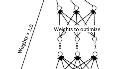
Incorporating given knowledge as a fixed input into a learning algorithm is equivalent to having that information persist through to the final output with coefficient 1.0. Such an architecture for a neural network is shown in Figure I.

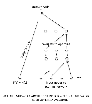
The neural network is effectively in two parts. One part passes the given knowledge unchanged to the end node. The other part is unconstrained as it may take on any structure needed to capture the full nonlinearity of the available data. The only additional constraint is that the output node must be consistent with the training of the given knowledge. In the case of our APC model, that was a logistic regression where the original G(v) function is being replaced with the learning part of the neural network. In the language of the neural network literature, that corresponds to a cross-entropy optimization.

III. NUMERICAL EXAMPLE

A. NeuralNetworks

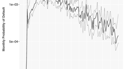
To demonstrate modeling the APC + neural network model, we used publicly available data from Fannie Mae and Freddie Mac on mortgage loan performance to predict mortgage defaults. The data was loan-level spanning a period from 2005 to 2017. The APC model was trained first on a vintage-level aggregation of the data using a Bayesian APC algorithm. The functions estimated were published previously [3].

Analogously to the multihorizon discrete time survival model developed previously [3], the lifecycle and environment functions were taken as inputs to the creation of a neural network as shown in Figure I. The input nodes included behavioral factors of credit score, LTV, loan purpose, etc. The inputs were measured monthly for each account. The output node would be used to predict the log-odds of default each month for each account. It is important not to threshold the final output node to a binary forecast. For mortgage defaults, almost all probabilities for default are less than 0.5, so thresholding would bias the forecast toward non-default.

In the tests on the mortgage data, this approach was effective at combining the given knowledge from the APC algorithm with the neural network. This was a test of effectiveness of the approach, not a specific attempt to out-perform the existing discrete time survival model. That said, the APC + NN model performed almost as well as the best-case discrete time survival model.

B. OtherDataMiningTechniques

Neural networks fit particularly well with incorporating probabilistic forecasts as given knowledge, because neural networks are a set of continuous functions. Many other data mining techniques are forms of discriminant analysis, where subsets of the input factor space are classified as discrete outputs. Decision trees, random forests, and support vector machines are all popular forms of discriminant analysis, but they do not employ any probabilistic or continuous functions that allow for the kind of direct integration as shown for the neural network.

Instead of integrating with the structure of the model, we can achieve the same goal by modifying the target data. Discriminant analysis techniques have long allowed weighting of observations by replication or deletion. Instead of assigning a continuous weight to an observation, significant observations can be replicated and insignificant observations can be deleted. To avoid losing observations entirely, the whole dataset could be replicated 100 times. Then according to some weights, remove some of the replicants or add even more replicants to other observations. The task then is to turn the given knowledge into a weighting scheme that can be applied to the training data.

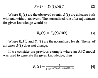
The mapping of given data to weights can be thought of as an adjustment from the observed level to the hypothetical level that would have been achieved if the data were normalized for the given knowledge. In a case of a binary target variable, take the observed rate as

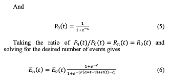
Therefore, the training data should be increased through replication or decreased through deletion to obtain the desired number of observed events.

The approach just described will allow for the creation of models on normalized data. That is equivalent to make forecasts for an average value of the given knowledge. However, this does not provide a mechanism for adjusting the forecasts for future values of the given knowledge. In the language of the loan default example earlier, this is a through-the-cycle model. Another method will be required to create forecasts with stressed scenarios.

IV. CONCLUSION

The modeling approach described in this paper solves a problem most likely present in every application of supervised learning to consumer behavior and other applications where long-term drivers are present on scales greater than the available data sample. The multicolinearity problem relative to long time scale drivers will not be apparent when only short-range forecasts are made, but product pricing, financial planning, and regulatory compliance all rely on long-range predictions.

The final solution of using a two-stage modeling approach and a specific architecture as shown in Figure 1 seems simple on the surface, but represents a dramatic change to how data mining is currently being applied in these areas. Getting the details correct for the architecture and activation functions creates the stability needed for long-range forecasting.

Further, the approach here of incorporating given knowledge can be used much more widely. The given knowledge could more generally be based upon business intuition or other non- model inputs. We intend to explore that further as it can expand the use of supervised learning into augmenting decision-making where full automation is not feasible.