Classical and quantum computing methods for estimating loan-level risk distributions

ABSTRACT

Understanding the risk distribution for a single loan due to modelling and macroeconomic uncertainty could enable true loan-level pricing. To implement such analysis, rapid real-time methods are required. This article develops a Monte Carlo method for estimating the loss distribution on classical computers. For this analysis, multihorizon survival models incorporat- ing the competing risks of default and pay-off were created on Freddie Mac data. The Monte Carlo simulation results fit well to a Lognormal distribution. Knowing in advance that a lognormal distribution is a reliable fit means that only tens of Monte Carlo simulations are needed to estimate tail risk in a single account forecast. We also explored the feasibility of using quantum computers that may be available in the near future to perform the calcula- tions. Leveraging previous quantum algorithms for value-at-risk estimation, we show that a simplified version of the problem has potential for significant speed enhancement, but the full competing risks approach will require additional quantum algorithm development to be feasible.

1. Introduction

When underwriting and pricing new loans, both consumer and commercial, the current best practice is to use forward-looking lifetime loss, payment, and yield projections using macroeconomic scenarios. Admittedly, most of the industry is not yet up to this best practice standard, but even the best prac- tice ignores the account-specific uncertainty in these forecasts. Uncertainty in the future loan perform- ance is left to economic capital calculations for the lender, or in best cases the product or perhaps major product segment. Scoring model uncertainties are regularly discussed in model validation. A wide range of additional business risks may be included, but a holistic treatment of account-level uncertain- ties is not being used for estimating account-level loss or yield distributions.

Account-level pricing cannot happen without account-level estimation of uncertainty. We believe the future of the lending industry is in using both the expected forward-looking cash flow forecasts for a prospective loan and the distribution of uncer- tainty about those estimates. In this article, we develop a method to estimate this distribution using Monte Carlo simulation on classical computers and explore how this can potentially be done faster on the quantum computers that will be available within a few years. The current hype around quantum computing is that it “will make everything run faster”. That is both untrue and largely irrelevant if the task at hand is offline, such as model develop- ment. For the lending industry, the greatest contri- bution of quantum computing may be in providing the real-time computation needed to facilitate preci- sion account-level underwriting.

Loan applicants can vary widely in their uncer- tainty. Two consumers with equivalent bureau scores could have very different performance uncer- tainties because of differences in the breadth and length of history available. The difference between success and failure for a lender can be in developing a practical understanding of where their underwrit- ing models are reliable and where they have excess risk. The model developer has much of this needed information about forecast uncertainty, but it rarely gets expressed other than in model documentation for review by validators. Instead, the lending indus- try needs to move to an underwriting process where lenders have ready access to account-level risk dis- tributions for lifetime loss and yield expectations.

To assess the account-level risk distribution in the context of a competing risks cash flow model, the following risks must be incorporated:

(1) Default risk score uncertainty
(2) Default risk lifecycle uncertainty at horizon h
(3) Default risk environment uncertainty at hori- zon h
(4) Prepayment risk score uncertainty
(5) Prepayment lifecycle uncertainty at horizon h
(6) Prepayment environment uncertainty at hori- zon h

This list of risks assumes that the default and prepayment scores incorporate only information known at loan origination, i.e. no behavioural attrib- utes. In the absence of behavioural attributes, the score estimation is separable from lifecycle and environment, but the lifetime loan profitability is not dependent only on the scores. Precisely when a loan defaults or prepays is also critical to estimating yield and the uncertainty in yield. The default and prepayment lifecycles measure the probability of default or prepayment as a function of the age of the loan, in this discussion referred to as the fore- cast horizon h. Lifecycles and their uncertainties may be estimated using survival analysis or Age- Period-Cohort (APC) models. The environment component refers to increased or decreased risk each month through the life of the loan. Macroeconomic factors are the primary means of modelling the environment. The environmental uncertainty comes from both the model estimation uncertainty and the uncertainty of the macroeco- nomic inputs.

For superprime loans, default risk will be low, but prepayment risk will be high, meaning that the effective life of the loan and uncertainty about that will be the biggest drivers of profitability. For sub- prime loans, default risk is high and prepayment risk is low, so uncertainty around default risk will be the biggest driver. Prime loans are impacted by all of these effects.

Current best practice is to use a “credit box” where they set boundaries within which they will originate loans in order to avoid regions of high uncertainty for the default and prepayment scores (if a prepayment score is employed). This credit box approach serves largely to control for the uncer- tainty where the credit score does not capture the tail risk of the loans. Environmental uncertainty is usually incorporated as the cost of funds for allo- cated capital Overbeck (2000); Carey (2009). Lifecycle uncertainty is rarely considered, and inter- actions between these risks on a monthly cash flow basis is never considered. The purpose of this article to consider the full set of uncertainties in a cash flow model and assess how to make this estimation process fast enough for real-time use.

Creating a lifetime forecast of anything that incorporates macroeconomic scenarios necessarily means that each time step will have a separate forecast with its own prediction interval, prediction intervals being a combination of the confidence intervals of the model coefficients and the error in the fit to the historic data. If we focus on predicting the probability of default (PD), then the prediction interval about the forecast will not be normally dis- tributed. Combining that with the complication of using a competing risks approach where the prob- ability of attrition (pay-off) is simultaneously pre- dicted means that error propagation cannot have a closed-form solution, nor do we have a matrix alge- braic solution that can be applied to Discretised distributions.

Monte Carlo simulation is the best available solu- tion to create the final distribution Glasserman et al. (2000); Binder and Stauffer (1984); Dupire (1998); Jaeckel (2002). At each time step, probability of default or attrite is drawn from their respective dis- tributions at that time step and combined with all other time steps in order to gradually tabulate the final distribution. Although effective, combining the full forecast distributions through all the time steps of a lifetime forecast is computationally intensive. Modelling challenges aside, the computation time has historically been an impediment to predicting account-level distributions for account decisioning. Speed issues are less important for such applications as estimating value-at-risk (VaR) at a portfolio level, but when employed for loan underwriting in a real- time environment, seconds matter.

Quantum computing is being promoted as the coming solution to computational speed limitations, but not all problems benefit or benefit significantly enough to matter when applied to quantum com- puters. Although few tests have gone beyond the proof-of-concept phase, the theoretical speed enhancements have been demonstrated in several areas. Shor’s algorithm for factoring integers is the earliest such success and captured headlines for its potential use in breaking encryption. Shor’s algo- rithm was enabled by the development of a quan- tum Fourier transform Weinstein et al. (2001), which can also accelerate any algorithm that would naturally employ FFTs. These methods provide greater than polynomial speed enhancements over current classical algorithms, but no proof exists that better classical algorithms could not be developed. In fact, quantum computing cannot solve any prob- lem not solvable via classical computing, and vice versa Nielsen and Chuang (2000). The question is one of speed, and in some cases insights from devel- oping quantum algorithms have created speed-ups in classical methods.

To understand where quantum computing may prevail, consider a computer with N binary registers (bits). An algorithm involving a series of basic operations could be applied to those N bits that sli- ces the problem into N pieces. With quantum com- puting, a set of N quantum bits (qubits) can encode 2N states, so instead of parallelising the algorithm N times classically, it is parallelised 2N times with quantum computing. If a classical CPU performed operations on 100 million bits of information simul- taneously, a quantum processing unit (QPU) would need only 27 qubits for the the same computation, in a perfect situation. The challenge is to find ele- ments of a problem that are parallelizable using quantum mechanical mechanisms of superposition, interference, and entanglement. Computers of the future may have a CPU, GPU, Neural Processor, and QPU to optimally solve different parts of the same problem.

The data science community has found several applications of quantum computing to accelerate the creation of models. These applications leverage the previously developed quantum algorithms for com- puting Fourier transforms and solving systems of linear equations. This includes quantum algorithms for performing principle components analysis Martin et al. (2021), creating deep neural networks Hu and Hu (2019) and convolutional neural net- works Cong et al. (2019), and support vector machines Rebentrost et al. (2014). Because Fourier transforms and solving systems of linear equations are foundational elements of many machine learning algorithms, many more accelerated algorithms are likely to be found. These will be particularly useful in contexts of creating models of massing data sets.

Several authors have demonstrated how quantum computing can be used in finance. Orus et al. (2019) with emphasis on option pricing Stamatopoulos et al. (2020); Martin et al. (2021).

Quantum computing can still be beneficial in applications where massive parallelism is not possible. Grover’s algorithm is a quantum search algorithm that can be applied to search an uncon- strained space in ffiffiffiffi N p steps where a classical algo- rithm would require N steps. This is not the exponential enhancement seen in the applications described above, but it is widely applicable in mod- elling and credit risk applications. Monte Carlo simulation is a natural use of Grover’s algorithm. Consequently, a quantum Value-at-Risk algorithm has already been proposed.

When considering possible applications of quan- tum computing, conceptually one could think of this as simultaneously computing on the full distri- bution of possibilities, but to record an answer, the qubits must be observed and a single answer obtained. Therefore, in the context of measuring account-level uncertainties, we can envision per- forming the computations across the full distribution at each time step, but the final answer will be a measurement of a quantity like the 95th percentile confidence interval on the lifetime yield.- may not be revolutionary in lending when so much time is spent on validation, documentation, and regulatory oversight before a model can go into pro- duction. However, if quantum computing could be used make some processes fast enough for real-time use, that may change the way lending is done.

Faster model creation is always useful, but credit risk model development is a slow, tedious process with many layers of review. The process is slow by design in order to minimise model risk around crit- ical forecast failures, fair lending compliance, audi- tor acceptance, etc. In a process that often spans years from data collection to deployment or months at the most nimble FinTechs, faster model develop- ment may not have as much impact on the industry as one would hope. One goal would be to use quan- tum computing to run the models built with clas- sical computers, replacing classical Monte Carlo simulation for uncertainty measurement with meth- ods based in quantum computing that can deliver the needed speed increase for real-time use.

In this article we develop a classical algorithm for measuring lifetime loan yield uncertainty, explore how this could be achieved with quantum computing, and along the way find methods to optimise the classic computation version sufficient for real-time use today.

1.1. Quantum computing basics

The basic computational unit for quantum computing is a qubit. As opposed to the 0 or 1 state of a classical transistor, each qubit represents a quantum system with an associated two-dimensional Hilbert space. The basis vectors of this space are written in the bra-ket notation of quantum mechanics as j0i and j1i, the x and y axes of our space. As a unit vector, qubits map easily to discussions of probability, because given a vector a b , the probability of obtaining either a 1 or 0 upon sampling the qubit is jaj 2 and jbj 2 , respect- ively with the condition jaj 2 þ bj 2 1⁄4 1:

To move beyond this weighted coin flip to encod- ing a full distribution, we use an m-qubit register (Klusch, 2003). Each individual qubit functions as above, but a set of qubits is used via a binary repre- sentation to encode 2m sample points along the prob- ability density function we wish to represent. The amplitudes of the register serve to bin the probability. For illustration, take m 1⁄4 2. With two qubits a b and c d , the tensor product creates four possible JOURNAL OF THE OPERATIONAL RESEARCH SOCIETY 3 states ac ad bc bd 2 6 6 4 3 7 7 5: Written in bra-ket notation, these states are j00i, j01i, j10i, and j11i with probabilities jacj 2 þ jadj 2 þ jbcj 2 þ jbdj 2 1⁄4 1: These four states can represent quartile sampling points of the binned probability density function. For greater computa- tional accuracy, meaning finer binning of the distri- bution, the number of qubits, m, is increased. During the calculations, the m-qubit register will maintain a superposition of all of these states. It will collapse to a single value only upon the final meas- urement, assuming a noiseless system.

An important consideration for later, is that quantum registers cannot be copied the way a clas- sical value is copied. If one of these m-qubit regis- ters is replicated, the two registers will be independent of each other producing different answers when sampled in the end. Said differently, two copies of an m-qubit register would encode the same distribution, but the final sampled answer will be two independent sampled values of those distributions.

Each time a quantum register is sampled, its quantum state is destroyed. This has important implications for how an algorithm is implemented. If a single quantum state is to be used in two separ- ate calculations, the two results are not independent. In classical computing the distribution can be sampled once, stored, and used in both calculations. In quantum computing the solution is to employ the quantum mechanical concept of entanglement (Penrose, 1998). With entangled copies, imple- mented with control gates on quantum computers, the final sample when performing one calculation will be identical to that used in a separate calcula- tion. The following example illustrates this principle.

Imagine randomly sampling two values, r and h in cylindrical coordinates and converting them to Cartesian coordinates as

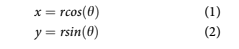
If r and h were were drawn from distributions and we wanted x and y to represent the final distri- butions of the conversion, r and h both need to be used twice in the calculation. If the r and h distribu- tions were sampled to compute x, that register’s state has been destroyed. It would need to be recre- ated and resampled, or copied and resampled to get values to use in computing y, but those would be different values, so the answer would be incorrect. In fact, if several calculations were to follow com- puting x and y, then the calculations should be performed on the registers without sampling until the end.

For example, imagine that x was to be incre- mented by one and then the angle recomputed,

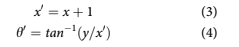
In a quantum computer, the circuit for perform- ing the calculations in Equations 1 through 4 should be performed without sampling until the end so that all operations are performed on the full distri- bution. At a high level, the quantum circuit would have the following steps:

(1) Load distribution for r into a quantum register
(2) Create entangled clone of quantum register for distribution of r
(3) Load distribution for h into a quantum register
(4) Create entangled clone of quantum register for distribution of h
(5) Compute x in new quantum register
(6) Compute y in new quantum register
(7) Add 1 to x
(8) Compute h0 in new quantum register

In the end, the quantum register for h0 holds a distribution of possible values. If only one value is needed, it could be sampled, but quantum superpos- ition will then be destroyed and cannot be reused without rerunning all the steps again. The full distri- bution cannot be read without performing some- thing like a Monte Carlo simulation where the the entire sequence above must be rerun for every sam- ple. Fortunately, quantum algorithms for Monte Carlo simulation have been developed to accelerate this process, and if only a desired point in the dis- tribution is needed, like the 99th percentile, acceler- ated algorithms have also been developed to extract that. Both will be discussed later.

In classical implementations of Monte Carlo simulation, the goal is to sample from possible com- binations of the relevant variables with probability given by the joint probability distribution. Imagine in the above example that the distributions for r and h were not independent. In quantum comput- ing, qubit will not hold a sampled value, but rather a superposition of possible states in the joint distri- bution. In a case of two distributions u and v, the superposition of possible states is written as jui jvi or in matrix notation as uvT: When we are con- sidering a sequence of time steps t 2 1⁄21, N, this leads to a superposition across an N-dimensional state space.

As a general rule of thumb, if the final answer can be represented as a single expression in matrix algebra, quantum computers can operate on this N- 4 J. L. BREEDEN AND Y. LEONOVA dimensional state space extremely rapidly as com- pared to a classical Monte Carlo simulation. Unfortunately, for the problem being studied here, no matrix algebraic solution is available. To find the final distribution for lifetime probability of default, the quantum algorithm for Monte Carlo simulation is needed.

Ironically, one could think of the potential speed- ups of quantum computing as a return to the analog computing of pre-transistor computation. Modern computers Discretised analog systems with high enough speed and precision that we forgot about analog computation. Being able to perform calcula- tions on a qubit with a continuous probability of values between 0 and 1 harkens back to those ana- log computations.

The above discussion covers the essential con- cepts needed for the current work, but for a more thorough introduction to quantum computing, see the appendices of Rebentrost et al. (2018).

2. Materials and methods

This article develops a real-world example by creat- ing models on US mortgage data using classical computing methods. From the lessons of that ana- lysis, we describe how this could be implemented on quantum hardware when that becomes available, along with scaling relationships for how fast that might be.

This method instantiation starts by building a long-range forecasting model following the multi- horizon survival model methodology (Breeden & Crook, 2020) for the probability of default (PD) and the probability of pay-off, a.k.a attrition, (PA) on publicly available Freddie Mac mortgage data. In developing the models, we are careful to follow the kind of rigorous development process expected by validation teams, with all confidence intervals cap- tured. The future environment is simulated with a second-order Ornstein-Uhlenbeck process Uhlenbeck and Ornstein (1930); Breeden and Liang (2015), like one might do for an economic capital calculation or lifetime loss reserves under IFRS 9 Stage 2 IASB (2014) or FASB’s Current Expected Credit Loss (CECL) FASB (2012).

Several sample accounts with diverse attributes were selected as test cases to be simulated classically via Monte Carlo simulation and then using quan- tum computing. This problem is actually beyond the capabilities of current quantum computers, so this is not a true head-to-head speed and features test, but rather a proof-of-principle to show how quantum computing can be employed in such a problem and what speed gains are expected relative to classical computing in the coming years as hardware catches up to this application.

2.1. Data

Data was obtained from Freddie Mac for 30-year, fixed-rate, conforming mortgages. The data con- tained de-identified, account-level information on balance, delinquency status, payments, pay-off, ori- gination (vintage) date, origination score, postal code, loan to value, debt to income, number of bor- rowers, property type, and loan purpose. Risk grade segmentation was defined such that Subprime is less than 660 FICO, Prime is 660 to less than 780, and Superprime is 780 and above.

The data in this study represents more than $2 trillion of conforming mortgages. The data made available by Freddie Mac is a large share of their portfolio, but not the entirety.

2.2. Forecasting model

Multihorizon survival models combine the age, vin- tage, time effects of an Age-Period-Cohort (APC) model Ryder (1965); Mason and Fienberg (1985); Glenn (2005); Breeden (2014) with attributes com- mon to behaviour scores, such as delinquency, bur- eau scores, loan-to-value ratios, etc.

The target variables are probability of default (PD) and probability of attrition (PA), a.k.a pay-off. Each of these probabilities is measured relative to the previous months’ active accounts in order to create a competing risks estimate Rutkowski and Tarca (2015).

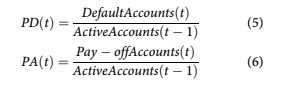
In this analysis, default is defined as any account that reaches 120 days-past-due.

Loan performance can be described in an APC model as

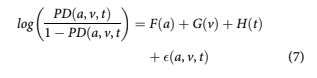
F(a), referred to as the lifecycle, measures the loan’s default risk as a function of age of the loan, a. The second function G(v) captures the unique credit risk of each vintage as a function of origin- ation date, v. The function H(t) measures variation in default rates by calendar date t to capture envir- onmental risks such as macroeconomic impacts.

These functions can be estimated via splines as in standard APC implementations or nonparametri- cally as in Bayesian APC Schmid and Held (2007). Although nonparametric estimation is appealing for the vintage and environmental functions, the Bayesian APC algorithms have proven to be less reliable when estimating confidence intervals about these functions. Considering the importance of con- fidence intervals in the current work, we have chosen a spline estimation with coefficients and confidence intervals estimated by optimising the maximum likelihood function.

Because the lifecycle, credit risk, and environment functions are summed, only one overall intercept term may be estimated. By convention, the estimates are constrained so that

The relationship t 1⁄4 v þ a also requires that an assumption be made about how to remove the lin- ear specification error. Consistent with earlier work Breeden and Canals-Cerda (2018), this is accom- plished using an orthogonal projection onto the space of functions that are orthogonal to all linear functions. The coefficients obtained are then trans- formed back to the original specification. We know from the work by Holford (1983) that once the con- stant and linear terms are appropriately incorpo- rated, the nonlinear structure for F, G, and H is uniquely estimable.

When the data is prepared for APC estimation, accounts may be censored based upon the account having previously paid-off, also called attrition. The probability of attrition (PA) is modelled analogously to the probability of default as

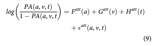
The functions obtained from APC analysis can measure vintage credit risk but not explain it. Therefore, to enhance the usefulness of the model and to better predict default, origination and behav- ioural information are added to the formulation.

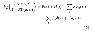
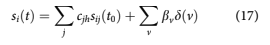
where sijðt0Þ are the available attributes on the fore- cast snapshot date t0 for account i. Such attributes include origination score, origination loan-to-value (LTV), and delinquency status, for example. The cjh are the coefficients to be estimated. Vintage dum- mies are still included with coefficients bv such that for a given v. To avoid colinearity problems between the APC and behaviour scoring components, the lifecycle and environment functions from the APC analysis, FðaÞ þ HðtÞ are taken as fixed inputs when creating a logistic regression model in Eq. 10.

In Eq. 10, t 1⁄4 t0 þ h where h is the forecast hori- zon 2 1⁄21, N where N is the end of the forecast. By including delinquency in the model, the coefficients cjh will change with forecast horizon, just as seen in the structure of a roll rate model or as would result from iterating a state transition model. Therefore, one panel logistic regression model is estimated independently for each horizon h.

In a stress testing context, the environment func- tion, H(t), would be correlated to macroeconomic factors Breeden and Thomas (2008). That introduces a difficult-to-quantify uncertainty around scenario generation. Since the goal here is to make the uncertainties explicit and incorporate them into the forecasting process, we elect instead to use a mean- reverting process calibrated to the history of the environment function.

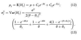
Following Breeden (2018)a2nd order Ornstein- Uhlenbeck process is created in order to estimate the distribution of H(t) in discrete time as

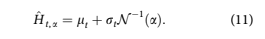
where a is the desired point in the distribution. The expectation values of mean lt and variance r2 t of Ht are

2.3. Classical Monte Carlo simulation

The forecast begins on a snapshot date t0. Using information available for account i at t0, we con- struct conditional distributions of the probability of default or attrition at each time t 1⁄4 t0 þ h where h is the forecast horizon.

In units of log-odds, all of the multihorizon sur- vival model coefficients represent the mean of a normal distribution of the possible values for those coefficients. The values for the environment H^ ðtÞ generated from the Ornstein-Uhlenbeck process are approximately normally distributed. Therefore, the conditional probability density functions can be expressed as

where a 1⁄4 t vðiÞ, v(i) being the account’s origin- ation date.

The account risk is obtained from the scoring component of the multihorizon survival model as

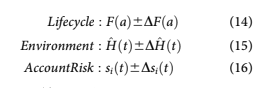
and DsiðtÞ is the confidence interval of the scor- ing prediction.

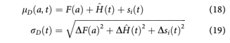
Since all of the forecast components in Eqs. 14 to 16 are normally distributed, the combined forecast is normally distributed /DðtÞ1⁄4NðlDða, tÞ, rDðtÞÞ where

and the probability distribution wDðtÞ for PD(t) will be a logit-normal distribution Mead (1965)

and the cumulative distribution function is

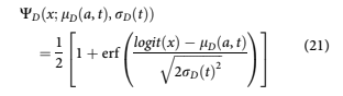
Similarly, we can obtain the distribution for the probability of attrition pAðtÞ at each time t as WAðx; lAða, tÞ, rAðtÞÞ: The distributions wDða, tÞ and wAða, tÞ are conditional on the account not having defaulted or attrited in any previous t 0 , t0 < t 0 < t:

For the Monte Carlo simulation, the conditional probabilities of default and attrition, PD(a, t) and PA(a, t), are randomly sampled from wDða, tÞ and wAða, tÞ: To obtain the unconditional probability of default or attrition at time t, UPDðt 1⁄4 t0 þ hÞ and UPAðt 1⁄4 t0 þ hÞ are computed as

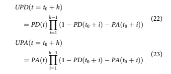
The final goal of the analysis is to compute the life- time probability of default LPD or attrition LPA as

LPD and LPA represent samples from the distri- butions fD and fA of possible lifetime probabilities, where lifetime is defined as N steps into the future. To understand the shape of the distributions, we need to propagate the logit-normal distributions through the calculation of UPD and accumulation to LPD.

The Monte Carlo simulation continues for each iteration j to generate samples for the conditional probability of default PDjða, tÞ from WDðx; lDða, tÞ, rDðtÞÞ and conditional probability of attrition PAjða, tÞ from WAðx; lAða, tÞ, rAðtÞÞ, which are processed via Eqs. 24 and 25 to produce the sampled values of lifetime default and attrition probabilities, LPDj and LPAj. The density functions fD and fA are then tabulated from these samples, although the primary interest for this article is fD, since eventually all loans pay-off that did not default, LPA 1⁄4 1 LPD:

2.4. Quantum Monte Carlo simulation

Every step of creating a forecast generates uncer- tainties. What we call a forecast is no more than the mean or median (depending upon the opti- mizer) of a distribution of all possible outcomes once we include everything we do not know or only know approximately. The Monte Carlo simu- lation used in classical computing is an attempt to tabulate that distribution piece by piece. Although the approach can be effective, it is notoriously expensive, so that practitioners never implement such systems in operational settings for lending. Offline simulations are used to understand the uncertainties generically, but this does not provide a borrower-specific answer.

Quantum computing algorithms for Monte Carlo simulation Kempe (2003); Aharonov et al. (2001) have been developed to provide substantial speed enhancement relative to classical Monte Carlo simulation. Although Quantum Monte Carlo seems like a logical name for such algorithms, that term is reserved for the simulation of quantum mechanical systems in physics and chemistry Ceperley and Alder (1986); Nightingale and Umrigar (1998).

Quantum random walk algorithms have also been developed Aharonov et al. (2001); Kempe

(2009); Yan et al. (2019), which might seem applic- able, but this problem is not one of a correlated random walk. The conditional PD and PA structure in Equations 5 and 6 means that all prior random draws PDðt0 þ iÞ and PAðt0 þ iÞ for i < h are uncor- related, but have a deterministic impact on UPDðt þ hÞ, not a statistical one.

The works of Egger et al., (2021) are directly applicable here. They created a quantum algorithm to run Monte Carlo simulations Montanaro (2015) for estimating value-at-risk (VaR). Their problem assumed a weighted sum of loss distributions for a set of assets from which a risk level such as 99.9% would be measured. In our case, we have a single asset, but a set of time steps to be summed. Determining the confidence interval about this fore- cast is equivalent to a 95% VaR calculation.

Therefore, we need to design a quantum algo- rithm, A that can be represented with three compo- nents. Following the notation of Egger et al. (2021):ƒ

• U Load the distributions UPD(t) onto N, m- qubit registers.
• S Sum the registers to a lifetime PD estimate.
• C Include a qubit for the condition that the value of the sum exceeds a test value x, here assumed to be the 95th percentile.

The operator C must be set for a specific signifi- cance value at the onset. Even though the quantum registers will encode the full final distribution being sought, only one point on that distribution may be measured with each simulation. Rather than running enough simulations to tabulate the full distribution, the goal is to determine the location of a single point.

The quantum algorithm is defined as A 1⁄4 USC: The key to making Monte Carlo simulation on quantum computers faster than a classical simulation is the use of a Quantum Amplitude Estimation (QAE) algorithm is applied (Brassard et al., 2002) to estimate expected values such as the 95% confidence interval, a. For QAE to work, A must be a unitary operator, which will be the case with the above structure. Let jwi 1⁄4 Aj0inþ1 denote the state obtained by applying A to the initial zero state for a register of n þ 1 qubits. Aj0inþ1 1⁄4 ffiffiffiffiffiffiffiffiffiffiffi 1 a p jw0inj0i þ ffiffiffi a p jw1inj1i for some normalised states jw0in and jw1in, where a 2 1⁄20, 1 is unknown, following the notation of Woerner and Egger (2019).

Applying QAE requires defining an operator Q 1⁄4 AðI 2j0inþ1h0j nþ1ÞA† ðI 2jw0inj0ihw0j nh0jÞ: The algorithm uses the samples from the Monte Carlo simulation to estimate the eigenvalues of the operator Q in order to efficiently estimate a, the probability that the last qubit will be 1. The eigenvalues are always sinusoidal functions, so a can be determined by applying a Quantum Fourier Transform Weinstein et al. (2001), or when the number of qubits is a power of 2, by applying a Walsh-Hadamard transform.

The returned value a is the cumulative probabil- ity from the distribution created by US relative to the test value x set as the threshold in C: To find the value x that corresponds to a desired value of a 1⁄4 a, an additional loop is created to perform a bisection search to find the smallest x such that the probability for a lifetime loss is less than a.

When estimating xðaÞ via a classical approach, the estimation is improved by a constant amount with each sample. The quantum algorithm encodes this information as an amplitude for which the esti- mation improves by a constant with each sample. Because amplitudes are squared to obtain probabil- ities, the accuracy obtained from a classical algo- rithm in M samples can be achieved with the quantum algorithm in ffiffiffiffiffi M p samples.

3. Results

The first step in the analysis was to create an APC model on the Freddie Mac mortgage default data. Then a multihorizon survival model was created with lifecycle and environment as fixed inputs from the APC decomposition. Lastly, a 2nd order mean-reverting model was applied to the environ- ment function.

3.1. APC decomposition

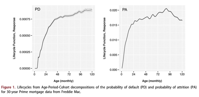
Figure 1 shows the APC decompositions for PD and PA. The PD lifecycle follows the expected pattern for prime borrowers, wherein the risk of default continues to rise relative to active accounts even for later ages, because of a selection bias where the low- est risk borrowers will eventually refinance or move. The environment function, shown in units of log- odds of PD relative to the lifecycle, shows mortgage default peaks from the 2001 recession and 2009 recession. The vintage function, also in units of log- odds relative to the lifecycle, shows previous periods of risky loans being booked prior to the 2001 and 2009 recessions. Although the most recent vintages have less data, the dramatic rise in credit risk from 2018 to 2020 is ominous.

The decomposition for PA shows that pay-offs are rare in the first year of a mortgage, but rising quickly. By 24 months-on-books, PA slows but remains high. As a consequence of this pay-off rate, the average life of a 30-year mortgage is closer to 7 years.

3.2. Score estimation

To estimate the coefficients of the multihorizon sur- vival model, a panel logistic regression model is created for each forecast horizon h with the previ- ously estimated lifecycle and environment as fixed inputs as in Equation 10. This was done for h 2 1⁄21, 12, because the most dynamic period is the first six months, and the coefficients largely reach satur- ation levels by horizon 12.

An essential part of the later analysis is that all coefficients include 95% confidence intervals. When the forecasts are created for the simulations, the pre- diction interval is computed about the forecast. The prediction interval incorporates the coefficient confi- dence intervals and in-sample goodness of fit. The confidence intervals for the coefficients and final prediction intervals are assumed to be normally dis- tributed in logit space.

The same process was followed for the probabil- ity of attrition, not shown here.

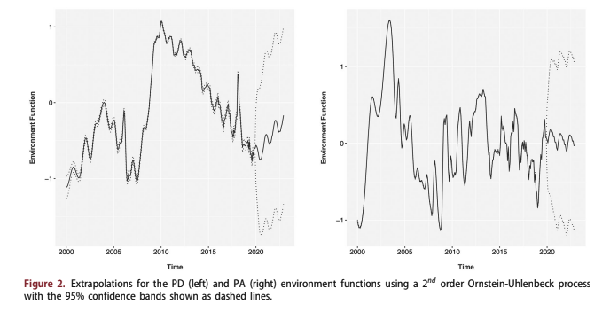
3.3. Environment extrapolation

As described in Section 2.2, the environment func- tions were extrapolated using a 2nd order Ornstein- Uhlenbeck process. This was done instead of the common stress testing approach of correlating the environment functions to macroeconomic factors. Examples of stress testing models for the environ- ment functions from Fannie Mae and Freddie Mac can be found in Breeden (2018). The goal of this analysis is to consider all possible paths for comput- ing a lifetime PD. Although a probabilistic model could in theory be applied to a stress test model rather than individual scenarios, that is significantly more difficult than going directly to a distribu- tional approach.

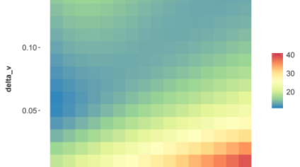
Figure 2 show the 95% confidence intervals for the environment functions under an O-U process.

3.4. Classical Monte Carlo simulation

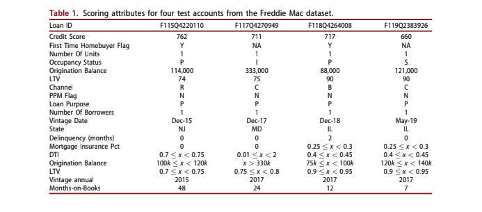
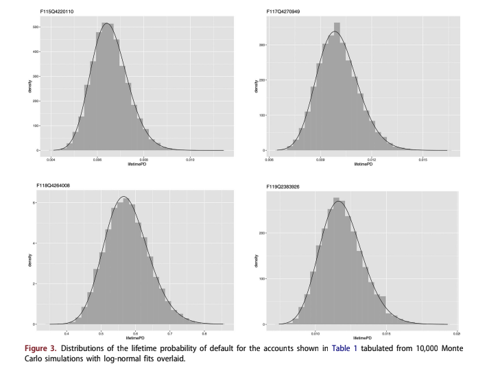
We ran a 36 month forecast from the last months- on-books of each account. Table 1 lists the loan attributes for four accounts specifically selected to have different risk profiles.

These accounts were predicted with the multihor- izon survival model under Monte Carlo random samples from the prediction intervals, lifecycle con- fidence intervals, and environment function extrapo- lation intervals to produce the results in Figure 3. 10,000 simulations were run to produce the smooth distributions shown. Lognormal distributions are fit to each account estimate, showing very strong vis- ual agreement.

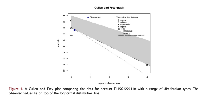
For each of these test accounts, a Cullen and Frey plot Cullen et al. (1999) was created to com- pare the distributions to a range of known types. Figure 4 shows one such example. In each case, the Lognormal distribution was the best fit.

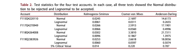
Table 2 provides three test statistics (Kolmogorov- Smirnov, Cramer-von Mises, and Anderson-Darling) for fitting Normal and Lognormal distributions to the simulated data Stephens (2017). The 5% critical values show that in every case, the Lognormal distribution was accepted, and the Normal distribution was rejected. This finding should be true as long as the probability of default is relatively low, so that the bound at LPD to 1⁄4 1 is not approached. That is true for typical loan applications and mostly fails only for severely delinquent existing accounts.

The effectiveness of fitting these distributions with a lognormal distribution is important. If we know before running the simulation that a lognor- mal distribution will be a good fit to the final distri- bution, we do not need thousands of simulations. Tens of simulations would be sufficient to estimate the mean and variance of the distribution in order to estimate the confidence interval about the forecast. When the number of Monte Carlo simula- tions was set to M 1⁄4 50, only 1.9 s was required to estimate the distribution for an account.

3.5. Quantum Monte Carlo simulation with unconditional distributions

The original motivation of this research was to determine if quantum computing could be used to compute entire distributions instead of laboriously tabulating them. The first things we discovered were that the competing risks approach outlined in Section 2.2 is deceptively complicated. The number of qubits needed grows, in the best case, linearly with the number of forecast steps and would use far more qubits than will be available in the next couple years given current trends. Therefore, this discussion of how quantum computing could be applied begins with consideration of a simplified case of uncondi- tional distributions for PD and PA and moves to the more complex case of conditional distributions.

Given hardware limitations for the near future, initial applications of quantum computing to account decisioning will almost certainly use single-risk mod- els. In the current context, this means directly fore- casting the unconditional probability of default at each time step, rather than considering the full com- pleting risks approach. The target variable, UPD(t), is redefined from the conditional probability of default in Equation 5 to an unconditional estimation

By modelling UPD(t) as a fraction of booked accounts, the attrition probability is implicitly incorpo rated into the PD modelling.

Nevertheless, this approach has the advantage in this context of making the distribution for PD at each time step t independent of the other time steps.

So, assume that this was done, and we have a direct expression for UPD(t) at each forecast horizon t 1⁄4 1, :::N and a logit-normal distribution wDðtÞ for which UPD(t) is the mean. A classical Monte Carlo simulation would randomly sample independently from the unconditional PD(t) at each time step and sum them to tabulate the final distribution. UPD(t) can be modelled with APC decompos- ition as was done before. Instead of the rising pro- portional risk for conditional PD shown in Figure 1, default risk will decrease with increasing age as fewer accounts remain from the original booked accounts. The UPD(t) environment function is a blend of the impacts to macroeconomic factors becomes

complicated as impacts from both default and pay-off are blended together. The overall result is suboptimal, but is found in use by some practitioners.

However, the combination with behaviour scor- ing as in the multihorizon survival approach is not available, because the panel logistic regression that is used to solve for the coefficients would need to include previously defaulted or paid-off accounts at every time step without censoring in order to pre- serve the denominator as booked accounts. Those post-default or post-pay-off accounts would be undefined in terms of behavioral variables such as delinquency or utilisation, so the regression becomes ambiguous.

To implement a quantum algorithm for estimat- ing lifetime UPD from unconditional distributions of UPD(t), we start by defining U, S, and C:

For operator U, the ability to load distributions efficiently into an m-qubit register is important and non-trivial. In direct estimation of UPD(t) without the competing risk framework, the distributions of UPD(t) at each time step will still be logit-normal distributions. Grover’s algorithm Grover and Rudolph (2002) proves that any log-concave distri- bution An (1998); Gupta and Balakrishnan (2012) can be efficiently loaded, which includes the expo- nential and normal families. Log-concave distribu- tions have the property that @2 log pðxÞ @x2 < 0:

Our logit-normal distributions could be loaded efficiently as normal distributions in logit space. An inverse logit-function could be applied to transform them to distributions in probability space, but the states of the qubit would no longer be uniformly spaced. That becomes a problem, because each time step t distribution would then have different meas- urement points.

register is not log-concavity, but rather that an effi- cient classical algorithm exists to integrate the prob- ability distribution. Log-concave distributions are one well-known example of this, but in the future others may find an efficient algorithm for loading logit-normal distributions. Until then, we have a choice of inefficiently loading the quantum registers or having a mediocre approximation to the original distribution. Efficient loading means that m opera- tions may be used to load the distribution, rather than 2m:

As stated in Grover and Rudolph (2002), the actual condition for efficient loading into a quantum

One such distribution must be loaded into an m- qubit register for each horizon h of the forecast. For unconditional distributions, S is a simple sum of all the registers. The implication is that the distribu- tions for increasing h shift the distribution to reduce the risk of getting a cumulative probability greater than one, but it is not guaranteed. In the quantum calculation, that translates to excess probability accumulating at the maximum probability because of the lack of a competing risk framework.

As described in detail by Egger et al., the key benefit to quantum computing comes from the speed gain in the QAE algorithm for obtaining expectation values. Every application of QðA corre- sponds to one quantum sample. QAE allows us to estimate the confidence interval for a with an esti- mation error that is bounded by

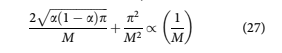
where M is the number of quantum samples. When compared to the / 1= ffiffiffiffiffi M p convergence rate of classical Monte Carlo methods (Glasserman et al., 2000), the speed increase is apparent.

Aside from speed, another feasibility consider- ation is the number of qubits required. For N time steps, N separate m-qubit registers are needed for the UPD(t) distributions. The QAE algorithm can be performed in-place using these m-qubit registers. Other qubits are required for parts of the estima- tion, but a toy problem could be implemented on existing quantum computers. from current computers could be largely noise because of these issues, but hardware improvements are being made quickly. Algorithmically, a solution is possible.

3.6. Quantum Monte Carlo simulation with conditional distributions

Our ultimate goal is to develop a system for estimat- ing the uncertainty in loan yield at underwriting. Consequently, the risk of prepayment is equivalently important to the risk of default, depending upon the demographic group. Adopting the full competing risks approach is significantly more complex than the correlated asset distributions considered in pre- vious quantum VaR work by Egger et al. (2021). Considering just one step in the calculation, Equations 22 and 23 can be written as

A key issue in the competing risks framework is that CPD(t) is used twice: once to compute UPD(t) and again to compute Sðt þ 1Þ: If we were to make a copy of the m-qubit register for CPD(t), the distri- bution would be preserved, but for the calculations to be correct, the two registers, the original and copy, must be perfectly correlated. The result is that the in-place register-saving calculations done for the summation in the previous step would no longer work. At each time step, two new registers for CPD(t) and CPA(t) must be loaded along with an entangled copy of the register for CPD(t). Entanglement in quantum computers is created via the use of con- trolled gates, e.g. CNOT gates.

Also, note that a register containing S(t) is used in calculation at every time step to compute UPD(t) and an entangled copy would be needed to compute Sðt þ 1Þ: If at each time step a quantum multiply operator M can be used to compute S(t) and then be repli- cated, the best case for the total number of registers needed for each quantum Monte Carlo sampling is 4 N and the number of qubits is 4Nm: This is a key point, because if the calculation of S(t) were not computed in place, the number of registers needed would grow exponentially with forecast horizon.

If we were simulating a five-year auto loan with an m 1⁄4 8 qubit register allowing 2m 1⁄4 256 bins in the probability distribution, the number of registers is 240 registers and 1, 920 qubits plus additional supporting qubits. That far exceeds the number of qubits available for commercial applications over the next couple of years and the number of compu- tations required via today’s hardware would reduce the result to noise.

The best path forward, for both the unconditional and competing risks versions of the algorithm is to know the shape of the distribution in advance. Just as this knowledge provides an advantage in the clas- sical Monte Carlo simulation, that information may be used to optimise the quantum algorithm. If we assume a lognormal distribution for the final answer, or generic beta distribution, the quantum algorithm for Monte Carlo simulation no longer needs to estimate a point in the tail of the distribu- tion, but can instead from estimated via as a closed- form calculation of the distribution’s parameters from a limited number of random samples. The QAE algorithm only needs to estimate the mean and variance of the distribution in order to obtain the necessary parameters for a lognormal distribution, which provides a substantial speed enhancement.F

4. Discussion

Model estimation uncertainties are rarely used in lending beyond validation, yet two loan applicants with the same modelled score could have very dif- ferent uncertainties depending upon the attributes that combined to create those scores. Although claims of loan-level pricing abound in the industry, prediction intervals and environmental uncertainties are almost never incorporated into underwriting and pricing decisions.

The goal of this work was to develop a frame- work using the best available forecasting models to create account-level distributions of lifetime prob- ability of default, and to implement this in a frame- work with the computational efficiency necessary to be part of a lender’s real-time decisioning. Our final run time using Monte Carlo simulation on a clas- sical computer of 1.9 s is clearly fast enough for real-time use.Although the model was complete, it covered only the lifetime probability of default. Incorporating bal- ance dynamics, revenue, and expenses would be needed to get to an estimate of yield and uncertainty in yield. Adding those pieces may cause the distribu- tion to no longer be a good fit to lognormal or beta, in which case our classical Monte Carlo shortcut would not work.

When starting the project, we did not know that a lognormal approximation would be possible, so our starting assumption was that a full classical Monte Carlo simulation would be too slow for real- time use. To address that possibility, we wanted to look at the promise of quantum computing. Although the available hardware can only run sim- plified problems, rapid advances are being made, so it would not be premature to explore what will be possible with quantum computing in the next cou- ple years.

ple years. To that end, we were also able to demonstrate that algorithms do exist for simulating a model that folds the estimation of probability of default and probability of previous survival (not previously defaulted or attrited) into a single model. Such algo- rithms should show a speed enhancement relative to classical algorithms on the order of the square root of the number of simulations needed.F

Lastly, by going through this detailed exercise, we were able to show that the full competing risks simulation using currently available quantum algo- rithms requires a large number of quantum regis- ters. That requirement pushes such an approach some years into the future. Instead, further research should be conducted to determine if a quantum cir- cuit can be developed to perform these calculations in-place with a relatively small number of qubits and if faster load times can be achieved for realistic distributions in credit risk applications.