Impacts of Drought on Loan Repayment

Abstract

In order to stress test loan portfolios for the impacts of climate change, historical eventsneed to be analyzed to create templates to stress test for future events. Using the 2012 MidwesternUS drought as an example, this work creates a stress-testing template for future droughts. Theanalysis connects weather and crop yield data to impacts on local macroeconomic conditions bycomparing drought-impacted agricultural counties with nearby urban counties. After measuring thenet macroeconomic impacts of the drought, this was used as an overlay with existing macroeconomicstress models to stress test a lender in a different part of the US for possible drought impacts. Havinga library of such climate events would allow lenders to stress test their portfolios for a wide range ofpossible impacts.

Keywords: climate change; drought; loan defaults; stress testing; age–period–cohort model

1. Introduction

Portfolio analysts often assume that stress test models must be created that are specificto climate change. The primary goal of this work was to demonstrate that climate stresstests could be performed using existing macroeconomic stress test models with the climateimpacts translated to macroeconomic scenario overlays.

In addition, although a significant number of analyses have involved the impact ofdestructive events such as hurricanes on property values, little investigation has been madeinto indirect impacts. By looking at how a severe drought can impact the local economyand lead to loan defaults, we demonstrate the importance of such indirect impacts evenwhen no property damage has occurred.

Section 2will provide background on the 2012 drought and the broader context ofclimate impact stress testing. Section 3describes the data used in the study and the sequenceof analysis connecting rainfall to crop yields to macroeconomic impacts to simulated loanportfolio losses. Section 4presents the analysis for selected counties that experienced thedrought, compared with the counties that were less impacted, and how this was used togenerate portfolio stress tests.

2. Literature Review

The 2012 Midwestern US drought has not previously been analyzed from the per-spective of loan portfolio stress testing. Therefore, the literature review was performedin two parts: a review of the conditions of the drought and a review of stress testing forclimate impacts.

    2.1. 2012 Drought

The years 2011 and 2012 saw a convergence of weather events, including a severeLa Niña (Boening et al. 2012) that brought dry conditions and a strong polar jet streamthat kept winter storms over Canada (Rippey 2015). These dry conditions were joinedby higher-than-normal temperatures through the summer of 2012. The severity of theresulting drought ranked second in the last 80 years behind the Dustbowl conditions ofJune to August 1936 (Schubert et al. 2004). These conditions severely impacted the yields ofcorn and soybeans (Lal et al. 2012). Even though the 2013 precipitation returned to normallevels, soil moisture at depths of 50 to 100 cm remained 18% below pre-drought levels(Bell et al. 2015)

Proving that any single event is a result of climate change is always difficult, but forthe purposes of simulating future events, the cause of past events is unimportant. Rather,we simply need to find past events that can serve as examples of how severe weathercan impact human livelihoods. This article examines the data from groups of severelyimpacted rural counties to show how the drought corresponded to drops in crop yields.With severely reduced real gross domestic product (RGDP), consumers in those countiessuffered job losses and falling property values. Consequently, those stressed economicconditions led to higher loan defaults.

The greatest difficulty in measuring the impact of the 2012 drought is that the USeconomy had not fully recovered from the 2009 recession, or in some cases, the rebound inpost-recession employment could mask the drought’s impacts. By looking at county-leveldata, the aggregations of rural counties were compared with the most populated urbancounties to measure the relative decrease in economic growth. The following sectionsshow the chain of events through such comparisons, quantify impulse functions for themacroeconomic impacts of the drought, and then demonstrate how these can be used in astress-testing context.

    2.2. Impacts of Climate Change

Climate change is clearly observable over the last century through both overt andsubtle events. These changes are severely impacting biodiversity and human habitabilityaround the world. With continuing carbon emissions and the feedback loops of melting icecaps (Jacob et al. 2012), permafrost (Kvenvolden and Lorenson 1993), deep-sea methane(de Garidel-Thoron et al. 2004), etc., humanity is unlikely to forestall future severe envi-ronmental degradation. Climate policy is critically important, but the question for thisresearch is the extent to which lenders must prepare for the impacts of climate change.

Climate change impacts on the banking system are broadly categorized as physicalor transitional (Alogoskoufis et al. 2021). Physical impacts are due to specific events orconditions that either damage the property that is used as collateral for loans or affect thebroader economy. Floods and hurricanes have been a focus of mortgage default modelingbecause of the obvious connection (Keenan and Bradt 2020;Kousky et al. 2020). Wildfireimpacts on mortgages have also been researched (Issler et al. 2020).

Property damage from hurricanes, floods, wildfires, derechos, or bomb cyclones canbe devastating to residents, but the collateral behind loans is usually insured. Insurancecompanies are appropriately worried about property damage, but this would not appearas the largest risk for lenders. Possibly, a greater risk to a loan portfolio would be whenthe borrowers’ livelihoods are damaged. In a hurricane, if the home survives or could berebuilt via an insurance claim, a consumer may still default on their credit card or auto loanbecause the local business where they worked was destroyed. Weather events that do notdestroy property, such as droughts and heatwaves, can similarly damage the local economycausing loan losses that are not covered by any collateral insurance. For these reasons, localeconomic damage is a greater risk to a lender than actual damage to collateral.

Transition risk refers to the costs to businesses and the economy in anticipation offuture climate events (Chakraborti and Gete 2021;Schütze 2020) or in response to complyingwith government mandates (Aguilar et al. 2021;Carattini et al. 2021;Semieniuk et al. 2021).

Transition risks are expected to be spread over multiple years, so although consumers andbusinesses may experience financial impacts, financial mitigation may be possible.

In consideration of the above factors, recent studies by banking regulators in theUK (Bank of England 2021) and EU (Alogoskoufis et al. 2021) have found only modestimpacts from even severe climate change. Part of this conclusion most likely comes fromthe system-wide perspective taken. National and multinational lenders are unlikely to beseverely impacted because of their geographic diversification. Rather, climate change riskswill be greatest for smaller lenders who are geographically concentrated. Quantifying therisks for smaller lenders is the primary motivation of this study.

3. Methods and Materials

The primary challenge in identifying the impacts of drought is the macroeconomicimpacts on those affected. Crop yield data are available by crop and county across the US.Quarterly macroeconomic data are available for US counties, but not all changes within theeconomy of a county are due to drought. The 2012 Midwestern drought was perhaps themost damaging to farmers since the Dust Bowl years, but this occurred during the recoveryfrom the 2009 Global Financial Crisis. Consequently, macroeconomic conditions were notsteady-state when the drought hit. Therefore, the best approach was to compare hard-hitcounties to those that were relatively unaffected, a control group.

This was accomplished by studying crop yields by county during normal years andthe presence of major cities. The counties that possessed major population centers withno consequential crop production were taken as the control group (urban). The countiesthat were major crop producers with low populations were put in the group of agricultural(Ag) counties. In comparing urban and agricultural counties, three states were chosen torepresent hard-hit, rainfall-dependent farmers, severe drought but with irrigated farms,and mildly affected farms, Table 1. By these criteria, the analysis of Kentucky is the mainpoint of this study with Nebraska and Minnesota serving as comparisons.

Table 1. A listing of top agricultural and urban counties for Kentucky (KY), Nebraska (NE), and Minnesota (MN).

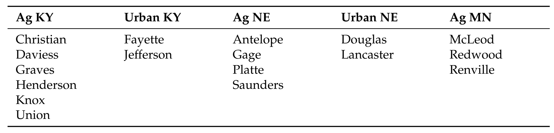
Kentucky’s corn-producing counties were chosen as the prime focus of this study because of how hard they were hit by the drought and the comparative lack of other economic activity. Nebraska’s soybean production was severely impacted by the timing of the drought and heat, but the state was less impacted overall because corn production was less impacted. Southern Minnesota corn-producing counties were only lightly impacted and thus serve as a control group. Because of the strong macroeconomic trends related to recovery from the 2009 crisis, Kentucky and Nebraska urban counties were compared in order to measure relative economic impacts.

Rainfall and crop yield data were compiled by Yun and Gramig (2019). County-level macroeconomic data were collected from the FRED website by the Federal Reserve Bank of St. Louis, https://fred.stlouisfed.org (accessed 20 June 2022). Loan performance data were available from FDIC call report data (FDIC n.d.). The stress testing example was performed on proprietary data from a California bank.

The analysis proceeded as follows:

1. Rainfall and crop yield data were reviewed to select county groups;

2. Aggregated macroeconomic series were created;

3. The differences between Ag and Urban counties were computed in order to measure macroeconomic impulse functions;

4. Drought impulse functions were overlayed on an existing macroeconomic scenario for a current portfolio;

5. Portfolio stress tests were performed using the adjusted macroeconomic scenario.

6. The first four steps provide the impulse functions that could be used by other an- alysts seeking to perform drought stress tests. The last step is an example of how the impulse functions can be used on an existing portfolio but is indicative only, not actual historical performance.

4. Discussion

    4.1. Precipitation and Crop Yields

The connection between precipitation and crop yields seems obvious, but rainfall must be neither too much nor too little and should occur at the correct point in the growing season. Figures 1–3 show the precipitation and crop yield data for Kentucky (KY), Nebraska (NE), and Minnesota (MN), respectively, (Yun and Gramig 2019). Although rainfall does not trend with time, crop yields show an obvious linear trend (Al-Kaisi et al. 2013). Based on a simple linear fit of the models to each state excluding 2012, crop yields in 2012 were predicted and compared with actual yields. Table 2 summarizes this analysis of the severity of conditions in 2012.

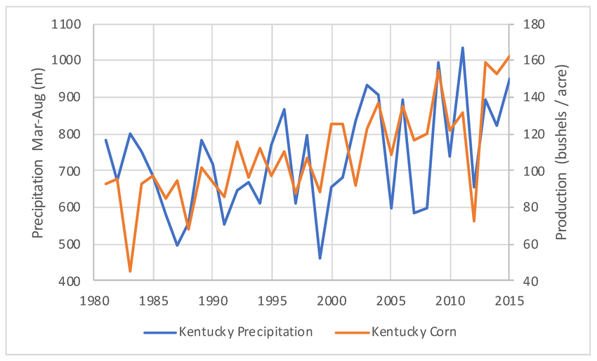
Figure 1. Precipitation and crop yield values for Kentucky, from “Agro-Climatic Data by County, 1981–2015”.

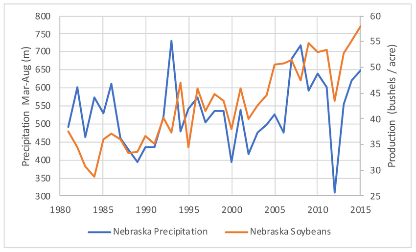
Figure 2. Precipitation and crop yield values for Nebraska, from “Agro-Climatic Data by County, 1981–2015”.

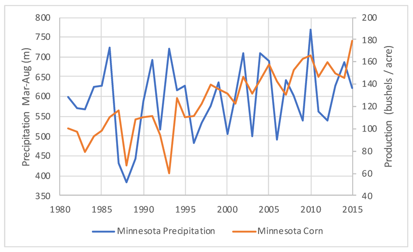
Figure 3. Precipitation and crop yield values for Minnesota, from “Agro-Climatic Data by County, 1981–2015”.

Table 2. A listing of top agricultural and urban counties for Kentucky (KY), Nebraska (NE), and Minnesota (MN).

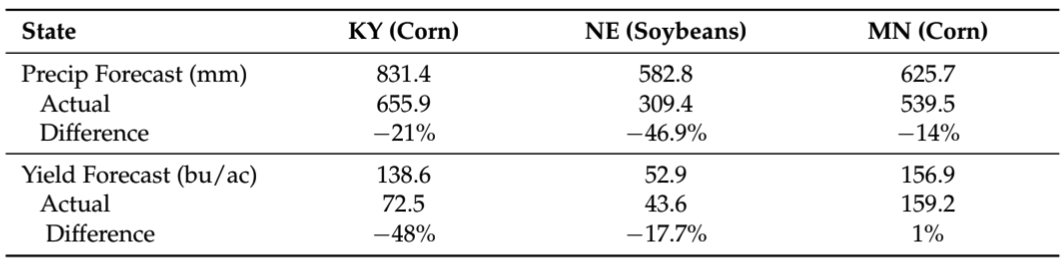
Even though Kentucky did not have the greatest drop in precipitation, the impact on corn yields was quite severe in an area with very little diversification. The drought in Nebraska may have been partially mitigated through irrigation. Minnesota showed a 14% drop in precipitation but no decline in corn yields.

    4.2. Employment

The next step is to quantify the connection between reduced crop yields and macroeco- nomic stress. Obviously, this will pose a hardship to farmers, but the broader implications for the local economy also need to be estimated.

Initial efforts to look for a rise in unemployment rates were less successful, presumably because those who lose their jobs in rural communities may relocate to urban centers to find work. A better gauge of job loss was to look at the change in employment. Figure 4 shows the year-over-year log ratio of employment growth, computed as

Log ratios are used here to measure growth, because the effects are additive, unlike percentage change. The comparison of agricultural to urban counties in Kentucky showed a dramatic divergence starting exactly with the drought. Agricultural counties continued to lag urban counties in employment growth for as much as five years following the drought, suggesting long-term harm to the economic base. Other than the drought, agricultural and urban counties showed remarkable similarities.

For Nebraska, the period in 2008 is curious and has the appearance of a data artifact. The 2012 drought may have contributed to lagging employment growth, but the signal is less clear, probably due to the greater economic diversity even in the agricultural counties.

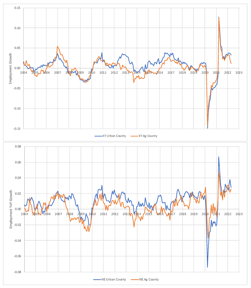
Figure 4. The year-over-year log ratio of employment comparing agricultural and urban counties in Kentucky and Nebraska.

Figure 5 shows the difference between agricultural and urban county employment growth, which shows that the drought signal in Kentucky is comparatively quite clear, aside from some noise.

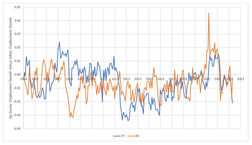
Figure 5. The difference in employment growth between agricultural and urban counties for Kentucky and Nebraska.

Figure 6 shows the creation of an impulse function that can be overlayed against future economic scenarios to simulate the impacts of a similar drought on employment growth. The agricultural minus urban county differences were smoothed the first year and extrapolated with a moving average thereafter via a straight-line approximation.

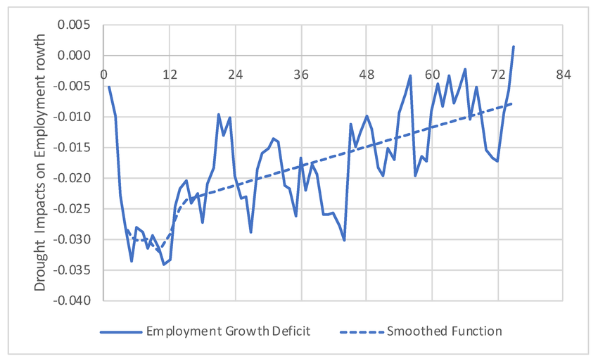
Figure 6. A smoothed impulse function for drought impacts on employment from the 2012 drought in Kentucky.

Minnesota is not shown in the above graphs, because the urban-to-rural distinction was just noise, as expected from Figure 3. The final impulse function was only computed for Kentucky (Figure 6), as we sought to understand the worst-case scenario in which irrigation was not available to moderate the drought.

    4.3. Zillow Home Value Index

If the drought causes a decline in employment, one could reasonably assume that property values would also decline. Zillow provides public information on typical home values via its Home Value Index (ZHVI), which is available at the county level (Zillow 2020).

Figure 7 compares home price growth for agricultural counties of Kentucky, Nebraska, and Minnesota. In addition, national-wide changes in farmland value were overlaid. Farm- land price data are provided by the USDA (Economic Research Service, U.S. Department of Agriculture 2020). The Minnesota ZHVI most closely tracked the USDA Farmland Value Index, with corresponding dips in 2009. The period from 2013 to 2022 showed a remarkable similarity in home value appreciation between all three states with the exception of Ken- tucky between 2013 and 2015. Shocks to local GDP and employment may have a lagged effect on home values, possibly explaining the delay to the beginning of 2013 for home values to fall.

Figure 8 shows a comparison of Kentucky’s agricultural and urban home value appre- ciation. Here the 2013–2014 deficit in home value growth is apparent.

Figure 9 shows the difference between the agricultural and urban home value growth rates to estimate a home value impulse function with the lag shown relative to the start of macroeconomic impacts for the drought in June 2012.

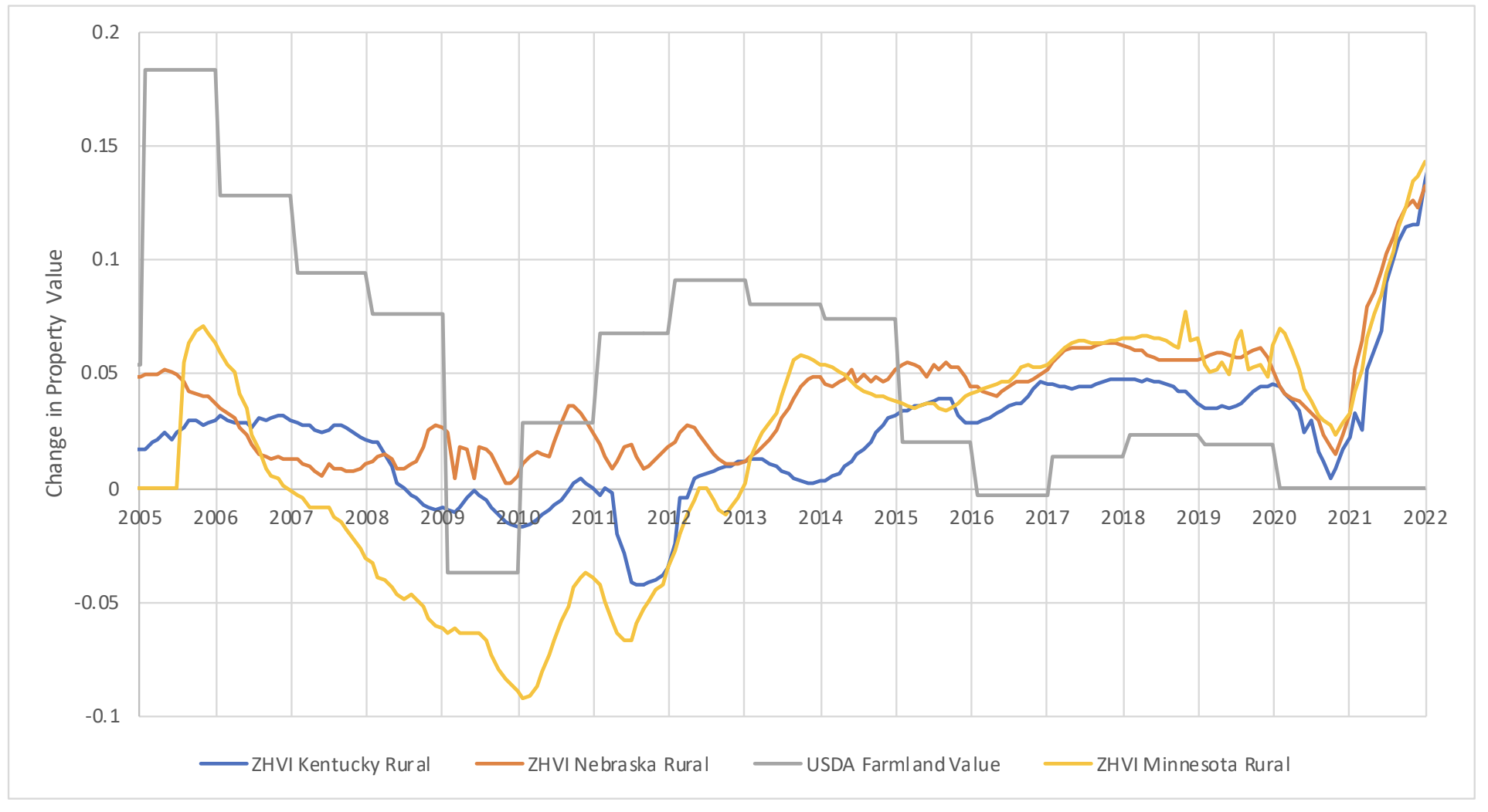
Figure 7. The year-over-year log ratio of Zillow Home Value Index for Kentucky, Nebraska, and Minnesota agricultural counties including an overlay of percentage change in the national USDA Farmland Value.

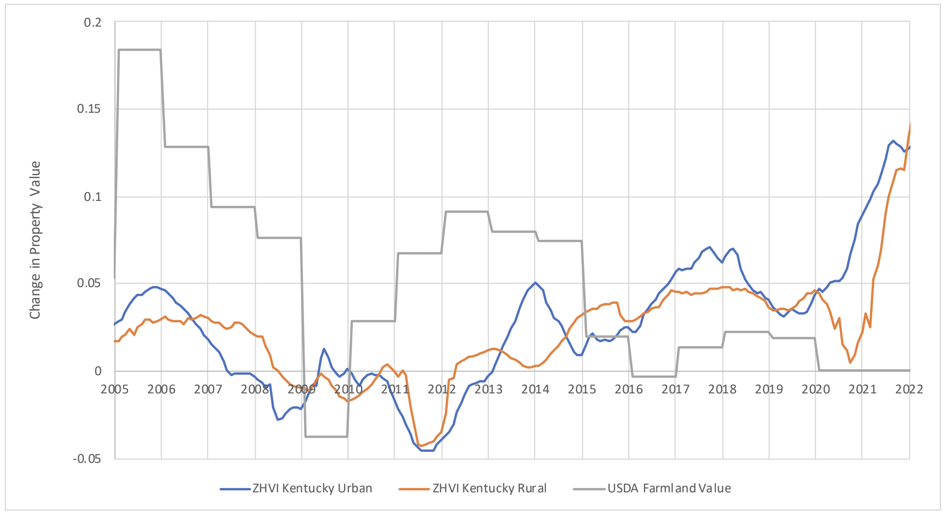
Figure 8. The year-over-year log ratio of Zillow Home Value Index for Kentucky agricultural and urban counties including an overlay of percentage change in the national USDA Farmland Value.

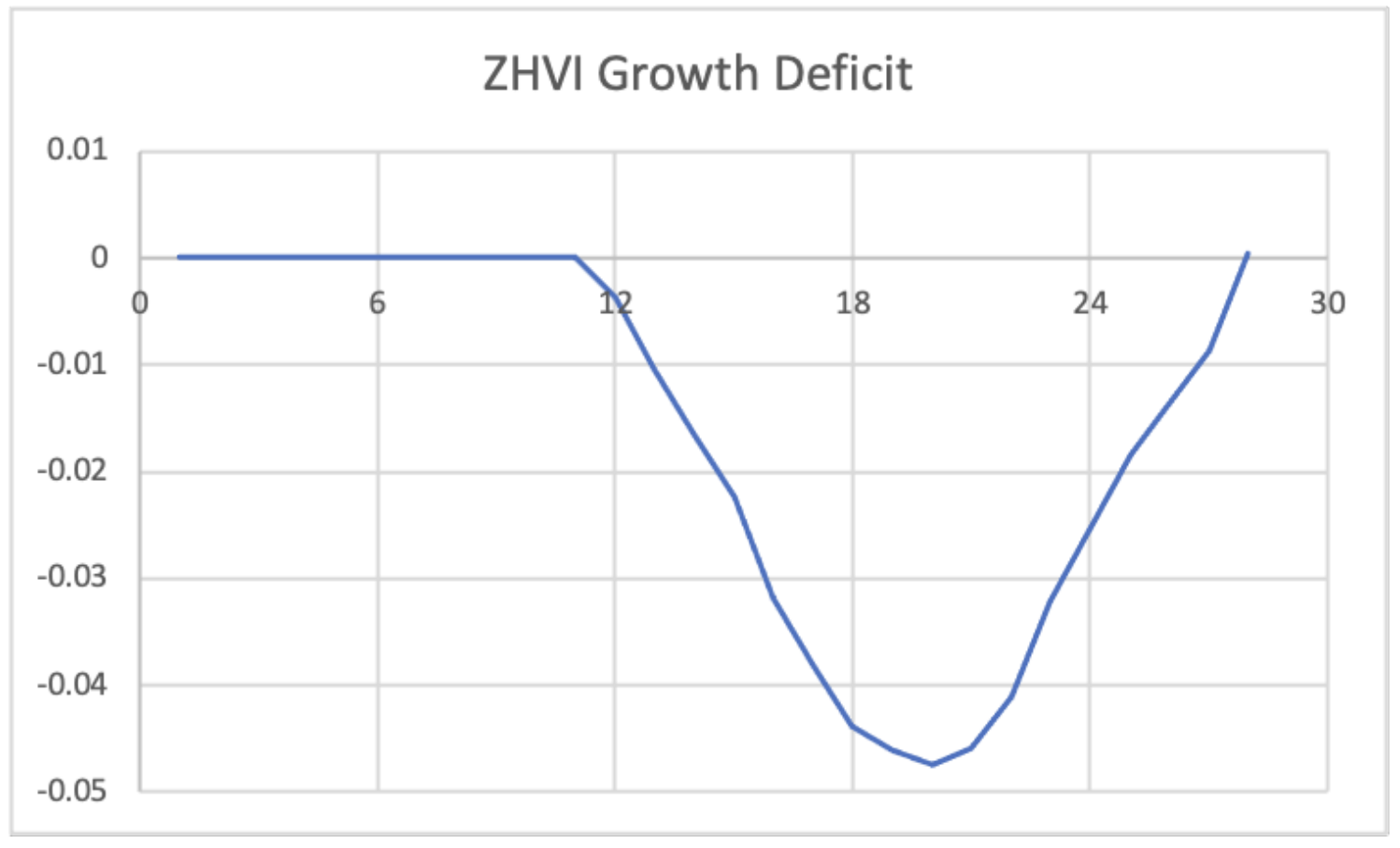
Figure 9. A smoothed impulse function for drought impacts on home value growth from the 2012 drought in Kentucky.

    4.4. Real Gross Domestic Product

Only a few macroeconomic measures are available at the county level. The quarterly reports of the real gross domestic product are available at the state level, but urban versus rural comparisons are lost in that case. At the county level, the RGDP is available annually, which trades time resolution for geographic resolution. Figure 10 shows the relative growth between agricultural and urban counties. Figure 11 shows the growth difference between agricultural and urban counties in Kentucky and Nebraska. Here again, Nebraska may show some impacts, but the signal is more clear for the Kentucky data.

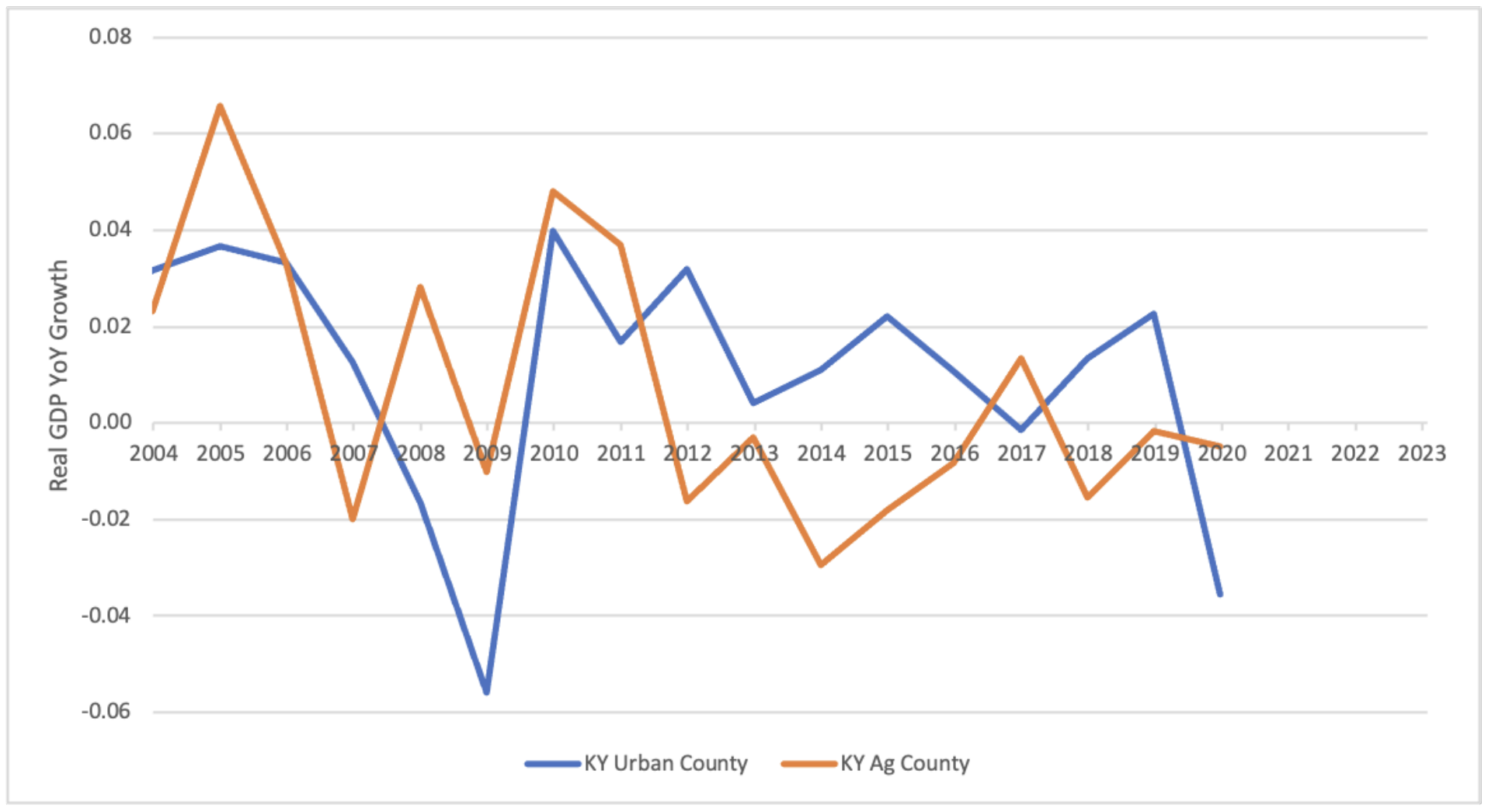
Figure 10. Annual log ratio of real gross domestic product for agricultural and urban counties in Kentucky.

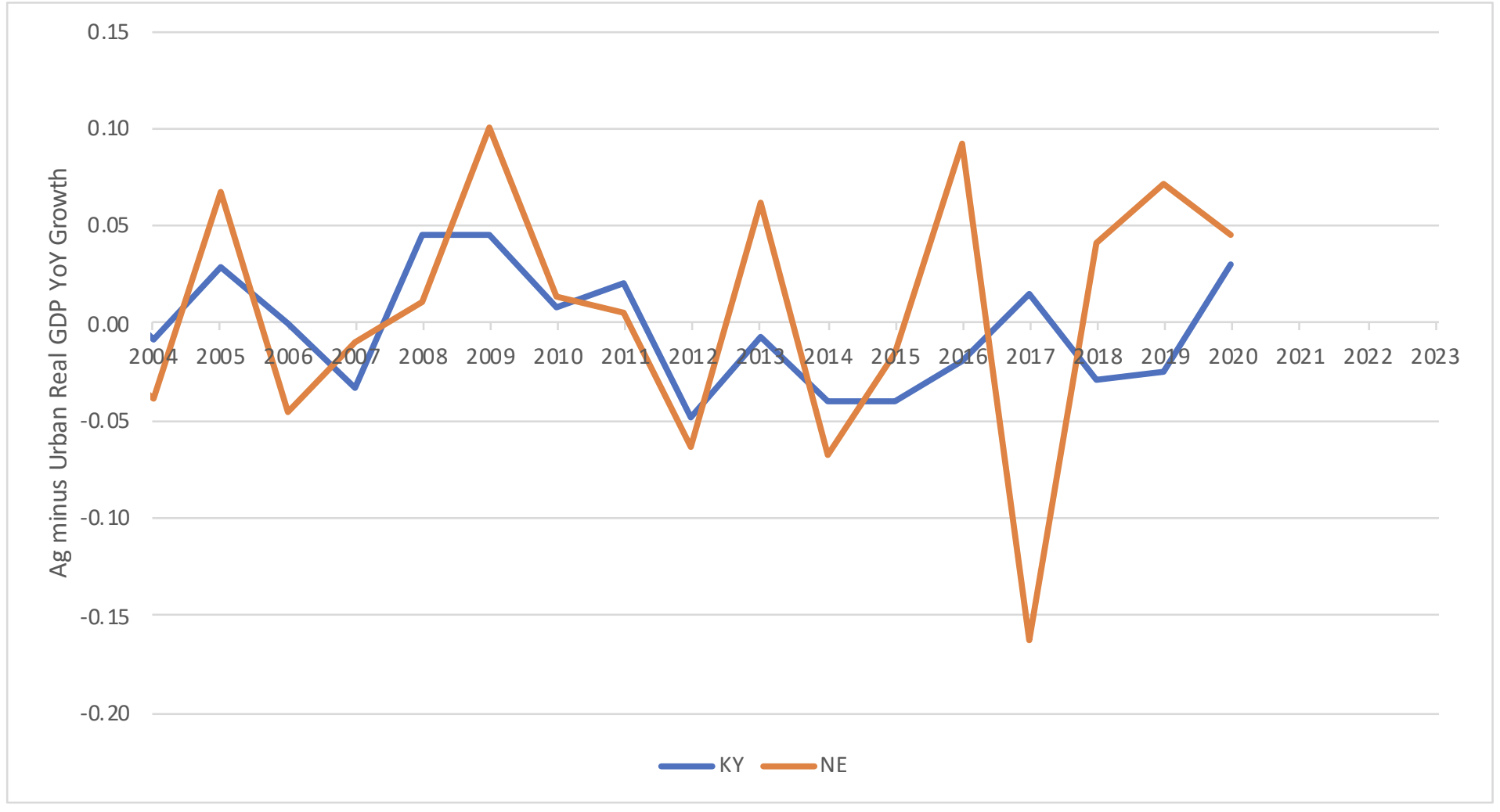
Figure 11. The difference in RGDP growth between agricultural and urban counties for Kentucky and Nebraska.

Figure 12 shows the impulse function created by smoothing the growth differences for Kentucky from Figure 11. This smoothing was performed such that the cumulative growth decline was preserved. These are admittedly weak signals within the broader macroeconomic environment, so smoothing is reasonable when creating a generalizable impulse function.

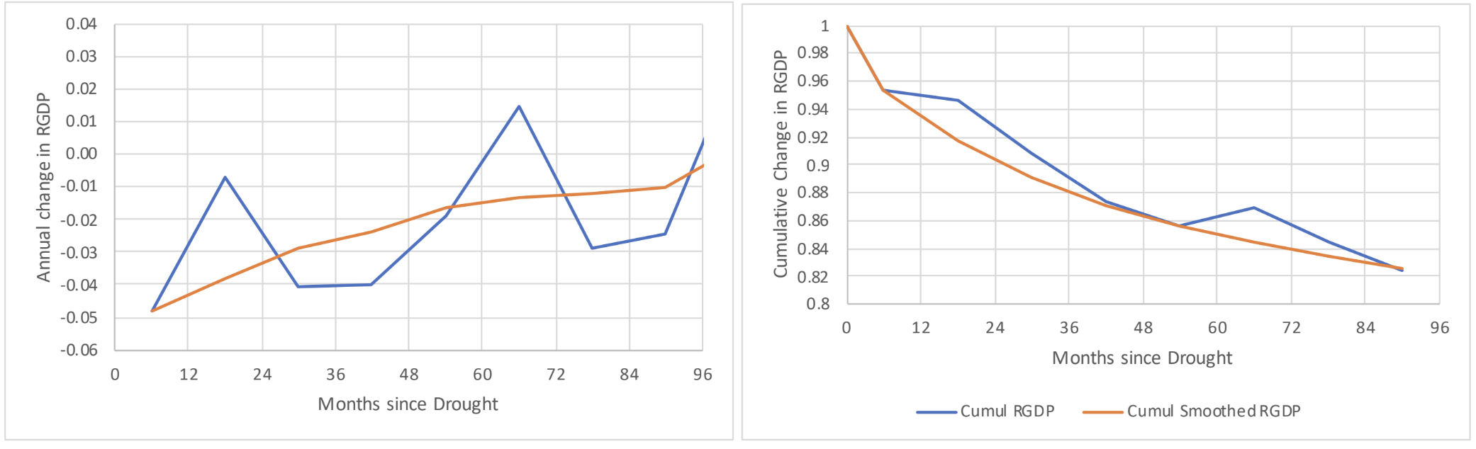
Figure 12. A smoothed impulse function for drought impacts on RGDP growth from the 2012 drought in Kentucky showing both annual and cumulative effects.

    4.5. Charge-Off Rates

Seeing macroeconomic declines in agriculturally focused counties is suggestive of future loan losses. Public account-level data are not available to directly test the connection between crop failures and loan defaults, but the Federal Deposit Insurance Corporation (FDIC) publishes aggregate loan-default data quarterly by major loan types (FDIC n.d.). Figure 13 shows the time series of the quarterly net charge-off rate for Kentucky, Nebraska, and Minnesota. Default is often recognized around 90 days delinquent, but charge-offs can be recognized with significant delays. The net charge-off rate is measured as charge- off balance net of collateral and cash recoveries divided by the outstanding balance in the previous quarter. Net charge-off rates can be negative, because recoveries may come in quarters subsequent to the initial loan charge-off, skewing the ratio. The broad peak centered on 2010 is assumed to be due to the 2009 recession.

The most notable second peak is seen in Kentucky’s agricultural lending in the upper left graph. Nebraska and Minnesota did not show a comparable increase, as Nebraska was more diversified, and Minnesota was only mildly affected.

The upper right graph of Figure 13 is for residential real estate loans. Kentucky and Nebraska showed identical improvements until 2012, where Kentucky showed additional mortgage losses not present in the other states. Unlike climate disasters, where the property is destroyed, these loan defaults were not covered by property insurance, so falling property values could impair recoveries, and net losses were realized.

The lower left graph for commercial real estate loans (CRE) and lower right graph for commercial and industrial loans (C&I) also revealed increases in net charge-offs even considering the relatively high noise levels in such low-event-rate products.

Net charge-off rates for consumer products such as credit cards and auto loans did not show clear patterns. Although consumer loans should have some connection to overall conditions, the connection is more indirect.

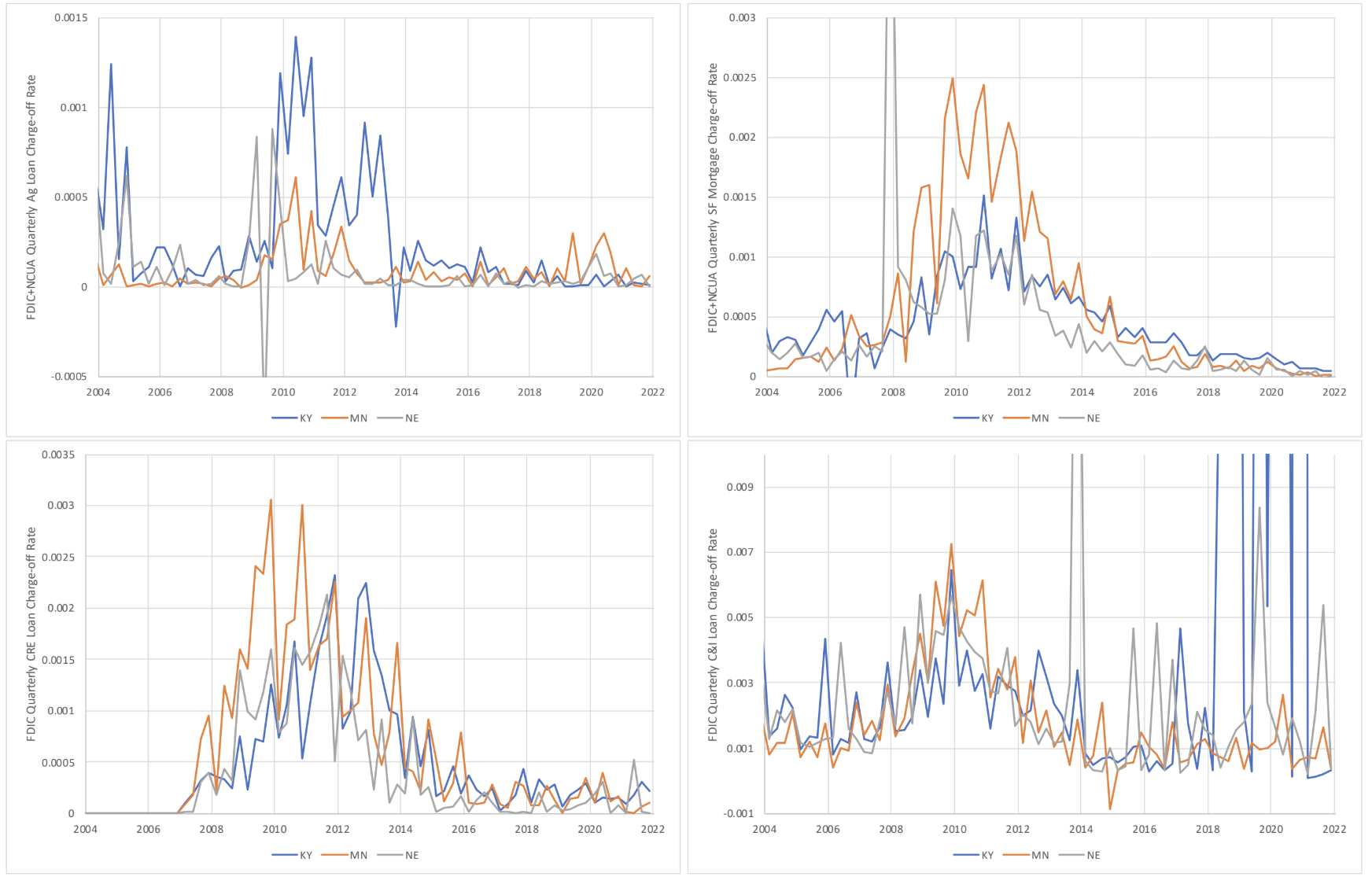
Figure 13. Net charge-off rate by product for Kentucky, Nebraska, and Minnesota.

    4.6. Stress Testing

The FDIC net charge-off data in Figure 13 suggested that the shock to Kentucky corn production caused loan defaults across several loan types. Given these data, one could create a model predicting net charge-offs by loan type in the FDIC data using macroeconomic factors or even directly from crop yield data. Although interesting, that is not the most useful for creating widely applicable simulations of climate change events. Rather than specifically forecasting climate-related futures, we adopted a scenario-based approach to explore the range of possibilities, such as those recommended by Ranger et al. (2022). This is also the recommended approach for modeling pandemic impacts, where disease impacts macroeconomic conditions, and the resulting macroeconomic scenarios were entered into loan portfolio stress test models. That approach was used to simulate epidemics from the Hong Kong SARS recession (Breeden 2014).

Macroeconomic scenarios appropriated to a given geography were created using a scaling of the impulse functions derived above as overlays to given macroeconomic conditions. Those scenarios can then be fed into existing loan default models to predict the impacts. Stress test models (Bangia et al. 2002; Berkowitz 2000; Committee on the Global Financial System 2005; FDIC 2014; Bellotti and Crook 2013, 2014) are widely available for larger lenders and from vendors for smaller lenders, so this allows any lender to quickly run drought scenarios.

The example from Kentucky corn production showed how an approximately 50% drop in corn yield impacted agricultural communities. This project began with a request from a lender in the California Central Valley who is concentrated in agricultural loans and associated CRE and C&I loans. Crops in this region are primarily irrigated, but a prolonged drought in the areas feeding the rivers to California would cause water restrictions where urban centers will likely be prioritized over agriculture. In this sense, the drought concepts are transferrable.

The greater difference was with the types of crops grown: tree fruits, nuts, and grapes. Severe water restrictions would not just cause the loss of a year’s harvest, but the loss of trees and vines as well. Replanting after such losses would cause the loss of three to four years of production. Therefore, the impulse functions from the 2012 Midwestern Drought need to be stretched to a longer-duration event, delaying the start of the recovery.

For the California Central Valley bank, age–period–cohort models were created for all of their loan types. The environmental functions were correlated to macroeconomic factors to create stress test models (Breeden 2014; Breeden et al. 2008). These vintage- based stress test models were used to predict the needed level of loss reserves under the current expected credit loss (CECL) framework (Breeden 2018). The CECL estimates were computed with a 36-month reasonable and supportable (R&S) period, meaning that only the first 36 months of the macroeconomic scenario were used in the forecast. Then, the environment was relaxed onto the long-run average environment for the remainder of the lifetime forecast. Consequently, even though the impacts of a drought might stretch beyond five years, only the first three years would be reflected in the forecast.

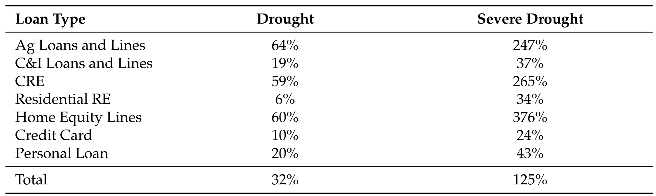
Table 3 shows the increase in net CECL loss reserve comparing a mild recession plus two levels of drought to a mild recession alone. The base drought is as described above. The severe drought increased the impact by 50%.

Directly overlaying the drought impulse functions on top of a mild recession scenario implies that the mild recession is driven by events that are independent of drought. In fact, at the time of this research, actions by the Federal Reserve to combat inflation were judged to create a high likelihood of a mild recession in 2023. Overlaying a drought scenario for 2023–2025 is not a specific weather prediction, but rather a stress test of what is possible given the extreme climate variability observed in recent years.

Table 3. Comparison of CECL loss reserves under mild recession + drought and mild recession + severe drought scenarios to a mild recession baseline scenario.

5. Conclusions

Quantifying the impact of drought on loan portfolios, particularly outside the direct impacts on agricultural loans, is notoriously difficult. The careful analysis design and county selection enabled the identification of this signal. Such analysis could be used to study other weather events where the signal-to-noise ratio for macroeconomic impacts is similarly low. Connecting this analysis to the use of macroeconomic stress test models that already exist at most lenders or are available from lenders makes climate stress testing accessible to a much broader group of lenders.

Stress testing is the most natural approach to assessing the possible impacts of climate change. Previous research has quantified the impacts of flooding, hurricanes, and wild- fires on mortgage lending. This article seeks to expand the library of impacts to include drought by focusing on communities that are economically sensitive to its impacts, namely agriculture.

Even in the areas most impacted by the 2012 drought, the signal can be challenging to measure because of recovery from the 2009 recession, uncertainty in the available macroeconomic data, and natural variability in human actions. Nevertheless, significant signals were observed, and the relative ranking of impacts in Kentucky, Nebraska, and Minnesota aligned with expectations.

In this study, we chose to perform a detailed analysis of the worst drought for which detailed data were available. However, it represents a single data point. Ideally, the same approach should be attempted on more localized droughts to see if confirming impacts can be measured and to enhance the statistical significance of the result.

The intention is that these results will be used to scale this drought event to other locations and events. Not all climate events can be modeled with this stress test library approach. The communities of the Florida keys would suffer severe, long-term impacts if a hurricane destroyed the Florida Keys Highway. Ski resorts and communities west of Denver would be severely impacted if wildfires and subsequent floods washed out sections of Colorado State Road 9. Such events are uniquely local and must be separately assessed both in likelihood and severity, probably via economic simulation rather than historical data analysis.

Overall, regional and community lenders bear the greatest risk from climate events. Being geographically concentrated can be part of the core value proposition of such lenders, such as being an agricultural lender in the Central Valley of California or a small business lender on the Gulf Coast. Therefore, such lenders must either add climate risk to their capital reserves or regularly sell parts of their portfolio in exchange for other investments in order to diversify their risk while continuing to generate profits from their domain expertise in that area.

Funding:This research received no external funding.

Institutional Review Board Statement: Not applicable.

Informed Consent Statement:Not applicable

Data Availability Statement:Economic and agricultural data are publicly available and referenced within the text. Example data for a specific loan portfolio were proprietary to the lending institution.

Conflicts of Interest:The author declares no conflict of interest.