Instabilities Using Cox Proportional Hazards Models in Credit Risk

Abstract

When the underlying system or process that is being observed is based upon observations versus age, vintage (origination time) and calendar time, Cox proportional hazards models can exhibit instabilities because of embedded assumptions. The literature on Age-Period-Cohort models provides clues to this, from which we explore possible instabilities in applying Cox PH. This structure occurs frequently in such applications as loan credit risk , website traffic, customer churn, and employee retention. Our numerical studies that are designed to capture the dynamics of credit risk modeling demonstrate that the same linear specification error from Age-Period-Cohort models occurs in Cox PH estimation when the covariates contain basis functions with linear terms, or if those covariates are correlated to the baseline hazard function. This demonstrates that the linear trend specification error in Age-Period-Cohort models is equivalent to multicolinearity instabilities in a Cox PH model or in any regression context when applied to comparable problems. As part of the multicolinearity studies, we show equivalences between Cox PH estimation methods and other regression techniques, including an original proof that Breslow’s method for Cox PH estimation is equivalent to Poisson regression in the case of ties.

Keywords: Data Science; Cox Proportional Hazards Models; Age-Period-Cohort Models; Poisson Regression; Conditional Logistic Regression

1 Introduction

Cox proportional hazard (Cox PH) models [20] have been used extensively in modeling consumer be- havior. Although Cox’s original development considered a hazard function with age combined with covariate information spread along another time dimension, consumer behavior actually exists in three time dimensions, age of the account a, vintage (origination time) v, and calendar time t. This structure includes the relationship that age equals time minus vintage, a = t − v. Such data sets are common in retail lending [8], fine wine prices [10], dendrochronology [17], website usage, employee attrition, and insurance underwriting [14]. The subject is particularly important for estimating credit losses for loans under the Financial Accounting Standards Board’s Current Expected Credit Loss (CECL)[26], International Accounting Standards Board’s International Financial Reporting Standards (IFRS 9) [33] and stress testing such as the US Dodd-Frank [19] and the Federal Reserve Board’s Comprehensive Capital Adequacy Review [25]. Nothing prohibits the application of the Cox model to observations in age, vintage, and time. How- ever, Age-Period-Cohort models [29, 32] were designed specifically for this three-dimensional analysis, and yet there is a well developed literature describing the specification error [31] that arises from the relationship a = t−v. The current article will explore the estimation properties of the Cox model when an age, vintage, and calendar time structure is present and more generally how multicollinearity affects the Cox model. In the process, we demonstrate the progression of estimation instability as certain features become more prominent in the data. This allows us to gain critical insights into the proper use of the Cox model, particularly in areas of heightened financial importance. These difficulties have been masked by the use of partial likelihood estimation in traditional Cox model estimation. Beyond the usual multicolinearity challenges present in any multiple regression model, the Cox model has a hidden multicolinearity problem between the time varying covariates and the hazard function. This analysis also sheds new light on the nature of the specification error in Age-Period-Cohort (APC) models. Rather than viewing this as a limitation of the model, it illustrates an inherent limi- tation in trying to fully specify systems that exist in these three dimensions from limited numbers of observations, regardless of the modeling technique. Depending upon the model used, this can appear as a specification error (APC), a multicolinearity instability (Cox PH and regression in general), or correlated residuals in lower-dimensional approximations (See Durbin-Watson [23] and Ljung-Box [35] in one dimension and Breeden [7] in two dimensions.) This article begins with a theoretical discussion of the consequences of multicolinearity when using different estimators for Cox PH models and related methods such as logistic regression and Poisson regression [34]. We discuss the equivalence between exact Cox PH estimation and conditional logistic regression, between Breslow’s method and Poisson regression, and between conditional logistic regression and unconditional logistic regression. Another original contribution of this paper is extending the literature on the equivalence between Breslow’s method and Poisson regression to the case of ties, which is a regular feature of observations in discrete time. Lastly we conduct a detailed set of numerical experiments designed to highlight the data features that cause Cox PH models to destabilize.

1.1 Background

Survival models [21] are an essential element in understanding the dynamics of processes in many fields. For loan portfolios, survival models could be applied to quantify the time to default as a function of the age of the loan, the time to attrition, the time to recovery, or several other potential loan events. As has been observed in previous portfolio analyses [4, 11, 6], loans within a homogenous segment will share a characteristic survival function, capturing the cumulative probability of surviving the specified event to a given time. The corresponding hazard function is the probability of an event like default occurring at a given time conditioned on not having occurred prior to then. We can also take the perspective that one test of a proper segmentation is that all loans share the same dynamical properties, such as following the same hazard function.

Cox recognized that not every ”unit” being tested for failure would have identical properties, so the hazard function could be scaled according to the unique risks of the unit. For lending, the analogy is clear. We expect a common hazard function for default probability also known as a lifecycle function or loss timing function, but individual loans could have higher or lower risk of default throughout the life of the loan based upon their attributes (credit bureau attributes, debt-to-income ratio, loan-to-value ratio for the collateral, etc.)

Cox’s solution was the proportional hazard model, or Cox model, as shown here.

λ(a, i) = e^xibλ₀(a) (1)

where λ(a, i) is the hazard rate for an event, λ₀(a) is the baseline hazard function, xi are a set of factors for loan i and b are the coefficients estimated to scale the unit relative to the hazard function given the input factors. With this formulation, the probability of survival to a given time t is

S(t) = exp ∫₀^t −λ(a, i)da (2)

Expressions of the Cox model typically refer generically to time of an event. We instead refer to the age a at which an event occurs in order to avoid confusion with macroeconomic effects by calendar date. In the language of lending, a ’score’ is created, xib, where the estimation of the coefficients is adjusted for the timing of the event. Did the event occur earlier or later than one might expect given the hazard function, and can that divergence be explained with available factors? Cox’s derivation involved the use of another innovation, the partial likelihood function. Since all loans would be subject to the same hazard function, this hazard function cancels out of the parameter estimation for the scoring coefficients. The consequence is that one can estimate the score without estimating the hazard function. To make forecasts of actual probabilities, both are needed but can be separately estimated.

To run numerical tests on Cox PH and understand in a broader context, we need to understand the methods available for estimating the parameters. These equivalences are not always well explained in the literature, so the following section provides proofs of the equivalences, which will be important later when we run numerical tests to draw conclusions about Cox PH. Cox PH exact estimation is equivalent to conditional logistic regression as discussed in Section A. Breslow’s method [12] is equivalent to Poisson regression with age as a factor as discussed in Section D[34, 18] . Conditional logistic regression is almost equivalent to unconditional logistic regression as discussed in Section E. Efron’s method has no regression equivalent.

Like Breslow’s approximation, Efrons method yields parameter estimates which are biased toward 0 when there are many ties (relative to the number at risk). However, the Efron approximation is much faster than the exact methods and tends to yield much closer estimates than the Breslow approach. When the number of ties is small, Efron’s and Breslow’s estimates are close to each other.

Age-Period-Cohort models [40, 36] are not being tested in this analysis, but the project was inspired by trying to understand the different assumptions between APC and Cox PH. APC models describe the available data with the sum of three functions. In the language of credit risk, these would be a lifecycle function versus the age of the account F(a), a credit risk function versus the vintage origination date G(v), and an environmental impact function versus calendar date H(t), such that

log-odds(Default) ∼ F(a) + G(v) + H(t) (3)

Because the data sets analyzed are typically uniformly sampled in time (monthly, quarterly, or annual), the functions are usually represented as a series of discrete points either smoothed (such as with splines) or nonparametric and estimated via maximum likelihood or Bayesian methods [39].

Only one constant term may be estimated among the three functions, and because of the relationship that a = t−v, only two linear terms may be uniquely specified amount the three functions. The second condition gives rise to the literature around specification errors. One can easily find examples, especially with data sets that are short relative to the dynamical cycles of the system, where all three functions should have linear terms and yet only two may be estimated or all three estimated by imposing an assumption. For example, mortgage loan portfolio from 2010 through 2018 might experience a long-term trend of improving economic environment, in response to which the lender books increasingly risk loans, and those maturing loans are increasingly risky with age because of a censoring effect where less risky loans pay off early. With only a fraction of an economic cycle, what should be part of a long-term cyclical process (economics and credit quality) appear mostly a linear trends.

One could create an equivalent Cox PH estimation where the G and H functions are estimated and no specification will occur. However, the estimation ambiguity is a property of the system generating the data, not the model creating the approximation. The APC literature proves that there is no colinearity problem in the estimation of F, G, and H aside from the linear specification [31]. However, the following numerical tests are designed to show that the implicit assumptions on the Cox PH model create estimation instabilities that originate from the same intrinsic ambiguity.

2 Methods

2.1 Theory of Multicolinearity

With regression models where all coefficients are estimated simultaneously, multicolinearity is straight- forward to understand theoretically and numerically. With Cox PH estimation, because the hazard function is not estimated or only estimated later when creating survival probability forecasts, multico- linearity is not easy to understand. For this reason, we study multicolinearity in a regression context and then demonstrate where Cox PH is equivalent to certain regression methods.

2.1.1 Multicolinearity in standard logistic regression

Logistic regression is a standard approach to modeling the kind of failure events for which Cox PH is usually applied [22]. The likelihood function is expressed as

L(β) = ∏^N_i=1 π^yi_i (1 − π_i)^1−yi, (4)

where

π_i = 1 / (1 + exp(−∑^K_k=0 x_ikβ_k)).

The goal is to estimate the K + 1 unknown parameters β in expression 4, typically using maximum likelihood estimation whereby the first and second derivatives of the likelihood function are estimated in order to identify the minima and maxima. The process is simplified by applying a logarithmic transformation to Equation 4.

Denoting l(β) = log L(β), then

∂l / ∂β_k = ∑^N_i=1 (y_ix_ik − π_ix_ik) (5)

∂²l / (∂β_k∂β_k0) = −∑^N_i=1 x_ikπ_i(1 − π_i)x_ik0 (6)

The β_b are estimated by setting each of the K + 1 equations in Equation 5 equal to zero and solving for each β_{b k}. The result is a system of K + 1 nonlinear equations with K + 1 unknown variables in each. Due to the complexity of solving this system of nonlinear equations, the most popular approach is to obtain a numerical solution via the Newton-Raphson method.

Using matrix multiplication, we can show that:

l′(β) = X^T(y − π), where π = (π₁, ..., π_N). Here l′(β) is a column vector of length K + 1 whose elements are ∂l / ∂β_k. Now, let W be a square matrix of order N, with elements π_i(1 − π_i) on the diagonal and zeros everywhere else. Again, using matrix multiplication, we can verify that

l′′(β) = −X^TWX (8)

The j step of Newton-Raphson can be expressed as:

β^(j) = β^(j−1) + [−l′′(β^(j−1))]⁻¹ · l′(β^(j−1))

Using Equations 7 and 8 the last equation can be written as:

β^(j) = β^(j−1) + [X^TWX]⁻¹ · X^T(y − π) (9)

If columns of matrix X are linear dependent (that is rankX < K + 1), then rank(X^TWX) < K + 1, the matrix X^TWX doesn’t have inverse and Newton-Raphson method so Equation 9 cannot be applied in this case.

Let rankX = K + 1. Due to the singular value decomposition

X = VDU^T,

where D = diag(√λ₀, √λ₁, ..., √λ_K) is a (K + 1) × (K + 1) diagonal matrix, where λ₀, λ₁, ..., λ_K are the eigenvalues of X^TX

V is a N × (K + 1) matrix, V^TV = I_K+1, and the columns v₀, v₁, ..., v_K of V are the eigenvectors of XX^T corresponding to the eigenvalues λ₀, λ₁, ..., λ_K+1

U is a (K+1)×(K+1) matrix, U^TU = I_K+1, and the columns u₀, u₁, ..., u_K of U are the eigenvectors of X^TX corresponding to the eigenvalues λ₀, λ₁, ..., λ_K+1.

Using singular value decomposition

[X^TWX]⁻¹X^T = [UDV^TWVDU^T]⁻¹UDV^T,

= (U^T)⁻¹D⁻¹(V^TWV)⁻¹D⁻¹U⁻¹UDV^T = UD⁻¹(V^TWV)⁻¹V^T,

= UD⁻¹V^TW⁻¹VV^T = UD⁻¹V^TW⁻¹

Hence the formula in Equation 9 may be written as

β^(j)_l = β^(j−1)_l + ∑^N_i=1 (y_i − π_i) / (π_i(1 − π_i)) ∑^K_k=0 (1 / √λ_k)u_klv_ki, l = 0, K, (10)

where

π_i = 1 / (1 + exp(−∑^K_k=0 x_ikβ^(j−1)_k)).

The situation when matrix X^TX is close to singular is called multicollinearity. The value

κ = √(λ_max / λ_min),

where λ_max and λ_min are the largest and the smallest eigenvalues of matrix X^TX, is called conditional number and is a measure of multicollinearity of the model. Traditionally, a rule of thumb has been suggested that values of κ that are 30 or larger indicate highly severe problems of multicollinearity. However, no strong statistical rationale exists for this choice of 30 as a threshold value above which serious problems of multicollinearity are indicated. [15]

From Equation 10 we can see that the larger κ is, the larger the resulting estimates β_b = lim β^(j) can be and the more unstable β_b can be to the small changes in covariates.

Case study. Consider vector functions F(a) = (F₁(a), F₂(a), ..., F_n1(a)), G(v) = (G₁(v), G₂(v), ..., G_n2(v)) and H(t) = (H₁(a), H₂(a), ..., H_n3(a)), which are sets of basis functions for the lifecycle, credit risk and environment functions correspondingly. And consider logistic regression model

logit(PD) = F(a)α + G(v)β + H(t)γ,

where PD denotes probability of default. The design matrix consists of columns F₁(a), ..., F_n1(a), G₁(v), ..., G_n2(v), H₁(t), ..., H_n3(t).

Assume that the set F(a) contains one constant and one linear function. Without loss of generality we can assume that F₁(a) = 1 and F₂(a) = a. Let G₁(v) = q₁v + r₁ and H₁(t) = q₂t + r₂. Since t = v + a

H₁(t) = q₂t + r₂ = q₂(v + a) + r₂ = q₂a + (q₂/q₁)(q₁v + r₁ − r₁) + r₂,

= q₂F₂(a) + (q₂/q₁)G₁(v) + (r₂ − (q₂/q₁)r₁)F₁(a).

Thus the columns of the design matrix are linearly dependent.

If under the same conditions F(a) consists of dummy variables for all unique ages, that is F(a) = (δ(a − a₁), ..., δ(a − a_n1)), then the design matrix is also singular since

H₁(t) = q₂a + (q₂/q₁)G₁(v) + r₂ − (q₂/q₁)r₁,

= q₂∑ⁿ¹_i=1 a_iδ(a − a_i) + (q₂/q₁)G₁(v) + (r₂ − (q₂/q₁)r₁)∑ⁿ¹_i=1 δ(a − a_i),

= q₂∑ⁿ¹_i=1 a_iF_i(a) + (q₂/q₁)G₁(v) + (r₂ − (q₂/q₁)r₁)∑ⁿ¹_i=1 F_i(a).

2.1.2 Multicollinearity in Poisson regression

Using the same reasoning we can show that in case of Poisson regression model multicollinearity can also cause huge parameter estimates, which can be also unstable (and even change the sign) to the small changes in training data.

The likelihood function for Poisson regression model is

L(β) = ∏^N_i=1 exp (−μ_i)μ^yi_i / y_i!,

where

μ_i = exp(∑^K_k=0 x_ikβ_k).

and log-likelihood is

l(β) = log L(β) = ∑^N_i=1 (y_i∑^K_k=0 x_ikβ_k − μ_i!).

The first and second derivatives are

∂l / ∂β_k = ∑^N_i=1 x_ik(y_i − μ_i),

∂²l / (∂β_k∂β_k0) = −∑^N_i=1 x_ikμ_ix_ik0.

The same derivatives in vector form are

l′(β) = X^T(y − μ),

l′′(β) = −X^TZX,

where Z = diag (μ₁, ..., μ_N) is a diagonal matrix.

Then the j step of Newton-Raphson method can be expressed as:

β^(j)_l = β^(j−1)_l + ∑^N_i=1 (y_i − μ_i) / μ_i ∑^K_k=0 (1 / √λ_k)u_klv_ki, l = 0, K

Thus, as observed in previous cases, as κ gets larger, the the resulting estimates β become unstable with small changes in the covariates.

2.2 Estimation Equivalences

The numerical tools available to study multicolinearity cannot penetrate the partial likelihood estimator employed in Cox PH models. To conduct experiments on Cox PH models, we need to use one of the panel-based estimators. We investigated the equivalence between various estimation procedures for survival models in order to establish the fidelity of these numerical experiements and their applicability to our understanding of Cox PH models. The appendix sections show where estimations are equivalent or nearly equivalent, so that the potential multicolinearity problems of the preceding section are seen to apply. Note that the proof of equivalence between Breslow’s method and Poisson regression is an original contribution.

Overall, these proofs and the numerical experiments below show that simulation is a valid approach to explore the stability of Cox PH models.

2.3 Numerical Experiments with Credit Risk Simulated Data

To explore possible instabilities in Cox PH estimation, we conducted a series of numerical experiments. The goal was to generate data sets from systems with known parameters and then use Cox PH to estimate the parameters with which the data was estimated. We want to identify systematic divergences between estimated and original parameters to within estimation error. Note that Cox PH always provides a unique solution, but convergence to a solution is not proof that the solution is correct. The question at hand is whether Cox PH can effectively estimate the original parameters. Simulated data is preferable to real-world data for this purpose, because we cannot know the true parameter values in real data sets.

The following tests unfold the multicollinearity problem in stages. First a single covariate model with correlation to the baseline hazard function is tested. Second we consider two factor models of different types, but without introducing all three dimensions of age, vintage, and time simultaneously. Lastly we look at the challenging but realistic situation with covariates both in vintage and calendar date.

Although the hazard function λ₀(a) is implicit in the Cox PH model, it is not directly estimated. For our tests, we focused on the estimates of coefficients for the covariates as provided by Cox PH. The hazard function was taken as a known input to the simulations and the estimation methods that assume it to have been previously estimated.

We use the following notation:

• Index i refers to an account (observation) i.
• v_i refers to the origination date (vintage) of account i.
• a and t refer to account age and calendar date at that age, respectively. Note that t = v_i + a.
• λ₀(a) is the baseline hazard for all accounts.
• x(i, a) is a predictor variable. It is a time-varying covariate (TVC) if x(i, a) ≠ x(i, b) for any i, a, b. Otherwise it is a static variable.

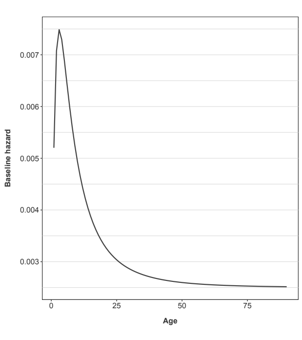
Figure 1 shows the hazard function used for the following simulations. It was created to mimic a shape that could be seen in default risk for consumer loan portfolios.

To simulate data for modeling, each of the following effects creates one or more predictor variables x(i, a). The probability of default is computed as given in Equation 1 for each forecast month. The coefficients b are set to 1 in all cases, so that we have an easily recognizable target answer. To simplify the interpretation of the results, no censoring (voluntary account closure) was incorporated.

For each of the tests below, 100 simulations with 10,000 accounts each, were generated. The start date, v_i, for each account is chosen uniformly across the 60 time intervals (months) of the simulation.

10

For each account, a default threshold was randomly generated with a uniform distribution [0, 1]. If the cumulative probability of default exceeds that account’s threshold in a given month, the end state is recorded and it is removed from further observations. The final data set contains the outcome event and any TVC values for the months up to the end state. All simulations end at 60 time steps (months).

Table 1 lists all of the tests considered. In the list below, Q(i, a) is an idiosyncratic risk scaling for account i, G(v_i) is the common risk scaling for all accounts originated in that vintage v, and E(t) is a common risk scaling for all accounts varying by calendar-date. Each of the tests is described in detail in the following sections along with the simulation results.

3 Results

3.1 Effect 1: Correlation to the baseline hazard

The first test is to generate data with a hazard function and a single TVC correlated to the logarithm the baseline hazard.

x(i, a) = (1 − δ)Q(i, a) + δ log λ₀(a)

such that 0 ≤ δ ≤ 1, and Q(i, a) and log λ₀(a) are uncorrelated, that is cor (Q(i, a), log λ₀(a)) = 0. The degree of correlation between x(i, a) and log λ₀(a) is controlled by a tunable parameter δ so that we may introduce correlation gradually through successive simulations. Q is a normally distributed random vector in 60-dimensional space.

A single-factor Cox PH model is estimated for each simulated data set. For a given value of δ, 100 simulations with 10,000 accounts each, were simulated as described above. The average relative error for estimating the coefficient b across all simulations is shown in Figure 2.

average relative error = (1/n) ∑_iⁿ |˜b − b| / b (11)

where ˜b is the estimated coefficient and b is the original value, which is set at 1 in all simulations.

3.1.1 Comparing Estimators

The coefficients and resulting error estimates were made with Breslow’s method, Efron’s method, and the exact method. In all cases the results from the three different estimators were practically identical, differing only on a scale well below the coefficient confidence intervals.

The near equivalence of these estimators is not a surprise in situations with plenty of data, such as here. The asymptotic efficiency of the partial likelihood estimator is investigated by Andersen, et. al. [3] and Fleming and Harrington [27]. On p. 315 of their book, Fleming and Harrington state, “In general, the partial likelihood based estimator of β will have high efficiency relative to the full likelihood

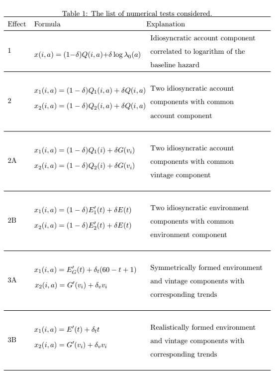
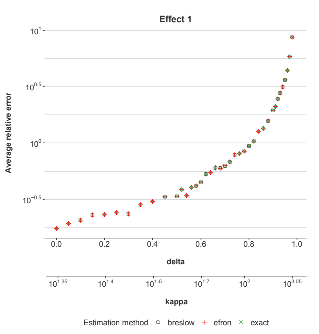
Figure 2: The estimation error in the coefficients for the explanatory factor x. Different tests were run with increasing correlation (δ) to the baseline hazard (λ₀). Kappa measures the level of multicollinearity within the data set.

approach if the ratio of the ’between time’ component to the ’within time’ component is small. The within time component represents the average (over observed failure times) of the variability of Z over a weighting of the risk set at each observed failure time, while the between time component represents the variability (over observed failure times) of the weighted average of Z over the risk set at each observed failure time.” It can be deduced from the formulae on page 315 that if covariates are independent from failure and censoring times then the estimations are equivalent. In our case all covariates are deterministic and therefore independent from default and attrition times.

Ren and Zhou [38] compare full likelihood estimation and partial likelihood estimation for small or moderate sample sizes. They conclude “...simulation studies indicate that for small or moderate sample sizes, the MLE performs favorably over Cox’s partial likelihood estimator. In a real dataset example, our full likelihood ratio test and Cox’s partial likelihood ratio test lead to statistically different conclusions.” The present study uses sufficient data that the differences are therefore irrelevant, so Efron’s estimator is used for the remaining tests.

3.1.2 Kappa

Conditional number kappa κ shown on the second x-axis of Figure 2 is a measure of collinearity in the model. Kappa uses the eigenvalue structure of X^TX where X is the design matrix, which includes columns for the X and log λ₀.

κ = √(λ_max/λ_min) (12)

where λ_max and λ_min are the largest and smallest eigenvalues of X^TX. Geometrically, kappa provides a measure of the shape of the data cloud formed by the predictors. The flatter the data cloud in some direction, the larger kappa is.

As δ increases, the multicollinearity increases, so κ also increases. As measured by κ, the multicollinearity increases exponentially with δ, so the error does also. Returning again to Figure 2, increasing values of δ causes increasing estimation errors. We have a multicollinearity problem in a one-factor Cox PH regression.

This is not just a toy problem. Modeling consumer loan defaults using a hazard function and delinquency as a predictor would be equivalent to this problem. For example, if delinquency were the TVC, kappa could be quite large as delinquency is strongly correlated to the default hazard function. Other uses of TVCs can be less correlated, but the available TVCs in lending applications could cover nearly the full range shown for kappa.

3.2 Effect 2: Two cross-correlated covariates

The next test simulates two cross-correlated covariates that do not have correlation with the baseline hazard. x1 and x2 each have idiosyncratic components Q1 and Q2 respectively, and a shared component Q controlled by δ.

x1(i, a) = (1 − δ)Q1(i, a) + δQ(i, a) (13)
x2(i, a) = (1 − δ)Q2(i, a) + δQ(i, a)

such that 0 ≤ δ ≤ 1, and log λ₀(a), Q(i, a), Q1(i, a), Q2(i, a) are pairwise uncorrelated random variables. Q1(i, a), Q2(i, a), and Q(i, a) are all normally distributed with mean 0 and deviation 1. The δ term controls the level of correlation between TVCs.

The data was generated as before and the estimation tests performed the same way. The results are shown in Figure 3.

In this example, x1 and x2 are symmetric, so the error estimates for their coefficients are also similar. The shape of the error function is a bit different from that in Effect 1, because the hazard function and Q have different distributions. So, the error scaling with δ is somewhat different, but the overall result is the same. The more correlated x1 and x2 are, the greater the estimation error. This example of multicollinearity is less surprising to practitioners than Effect 1, because both TVCs appear in the regression equation whereas Effect 1 involves multicollinearity to a factor (the hazard function) not in the regression equation.

3.2.1 Effect 2A: Idiosyncratic and vintage effects

We're now looking at a special case where the normally distributed random variable Q in Equation 13 is replaced with a **vintage effect, G(v_i)**. Each account is assigned a vintage based on its origination date, and all accounts within a given vintage share the same systematic risk factor, G(v_i).

This vintage effect is modeled as a stationary **AR(1) process**:

G(v) = 0.9G(v − 1) + N(μ = 0, σ = 0.25) (14)

The covariates x1 and x2 are then defined as:

x1(i, a) = (1 − δ)Q1(i) + δG(v_i) (15)
x2(i, a) = (1 − δ)Q2(i) + δG(v_i)

In this setup, Qj are not indexed by age but remain normally distributed. Essentially, Q(i, a) is replaced by G(v_i). Consequently, neither x1 nor x2 are truly **time-varying covariates (TVCs)** in this specific scenario. However, this model realistically represents accounts that have both a constant **idiosyncratic risk factor** and a **systematic factor** that depends on their origination month.

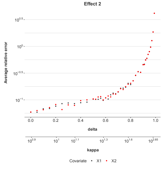
Figure 3: The estimation error in the coefficients for the explanatory factors xj for Effect 2.

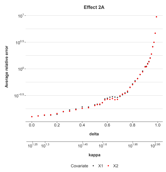
Figure 4: The estimation error in the coefficients for the explanatory factors xj for Effect 2A.

As shown in Figure 4, the estimation errors increase with δ even a little faster than in Figure 3. This shows that the factors xj need not be time varying for multicolinearity problems to arise.

3.2.2 Effect 2B: Environmental effects

We also consider a special case where the two cross-correlated time-varying covariates (TVCs) are **environmental variables**, meaning they are functions of **calendar time, t**. Each explanatory factor has an idiosyncratic component, E'_i(t), which varies with calendar time, and a systematic component, E(t), also varying with calendar time. It's important to note that while these are "time" varying, this dimension of time (calendar time) is distinct from the age-dependent hazard function, where age 'a' is defined as t - v (calendar time minus vintage).

The covariates x1 and x2 are defined as:

x1(i, a) = (1 − δ)E'₁(t) + δE(t) (16)

x2(i, a) = (1 − δ)E'₂(t) + δE(t)

In this setup, E'_j(t), E'_k(t), E(t), and λ₀(a) are pairwise uncorrelated. E'_j(t) are independent and identically distributed (i.i.d) random samples, normally distributed. E(t) is modeled as a full cycle sine function with added normally distributed noise:

E(t) = N(0, 0.4) + sin(2πt/60 + π) (17)

where t ∈ [1, 60] to simulate 60 months of data.

Figure 5 shows the results. The error levels in this case increase similarly to what was observed for Effects 2 and 2A. This demonstrates that the source of the collinearity can be at the account-level, vintage-level, or by calendar date, and the fundamental effect on estimation error remains largely consistent.

3.3 Effect 3A: Symmetric environment and vintage effects

Effect 1 showed that **factors correlated with the hazard function degrade estimation accuracy**. All variations of Effect 2 confirmed that **cross-correlation between explanatory factors also leads to degradation in accuracy**, even when these factors operate on different dimensions than the hazard function.

Effect 3A: Combining Environmental and Credit Risk with Symmetric Generation

In Effect 3A, we aim to combine both **environmental** and **credit risk effects** as distinct explanatory factors. To simplify interpretation, we're starting with an environment function that's generated using the same random walk process as G(v), with the key difference that E_G(t) remains a function of calendar date.

The relationship **t = a_i + v_i** inherently introduces a **linear specification error**. This is because the hazard function, the environment function, and the credit risk function can all potentially include linear trends.

The explanatory factors are defined as:

x1(i, a) = E_G(t) = E'_G(t) + δt(60 − t + 1) (18)

x2(i, a) = G(v_i) = G' (v_i) + δv_iv_i

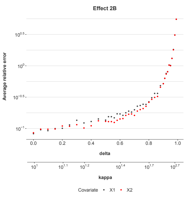
Figure 5: The estimation error in the coefficients for the explanatory factors xj for Effect 2B.

Assuming both variables are centered at zero, without loss of generality, and cor (E'_G(t), t) = 0 and cor (G'(v), v) = 0; i.e. E'_G and G' have no linear trend. The terms δ_t and δ_v allow us to control the amount of linearity in the functions. Note that the hazard function will introduce a non-zero linear component versus age 'a', which will also conflict with either of the linear components in Equation 18, even if one of the δ_t = 0 or δ_v = 0.

Equations 18 do not introduce multicollinearity as normally defined for Cox PH, but are designed to show how a linear specification error between different dimensions is translated to a multicollinearity problem.

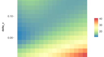
As can be seen in Figures 6 & 7, even small amounts of added linear trend cause a rapid increase in multicollinearity, κ, and a rapid increase in the estimation error of the coefficients. Equations 18 were designed so that the linear trend component would be tunable and demonstrate how sensitive the result is to this form of multicollinearity.

The functions in t and v were constructed to be as symmetric as possible. Each randomly generated G' (v_i) was replicated to E'_G(t) for that simulation. The linear trend in t was inverted so that it would exactly match the trend in v. However, all of this effort was not enough to produce identical estimation results for the estimated parameters. A careful review of Figures 6 shows that the scale is smaller for the error in x1. The issue is apparently the censoring that occurs because default is a terminal state. A truly symmetric data set is not possible, but the results prove the point that any small amount of linear trend makes the estimation unstable.

Although results from Efron’s method are shown, they are nearly identical to Breslow’s method (Poisson regression). This is relevant because for Breslow’s method, the hazard function is estimated as a nonparametric function simultaneously with the coefficient estimates for x1 and x2. If instead of x1 and x2 we were to directly estimate coefficients for t, E'_G(t), v_i, and G' (v_i), a singular matrix error would occur, because the linear trends conflict with the hazard function estimate.

Effect 3 demonstrates that the trend specification problem for age, vintage, and time appears in Cox PH estimators as a multicollinearity problem and in Age-Period-Cohort models as a specification error, but they are the same problem. It occurs because of the structure of the system generating the data being modeled.

3.4 Effect 3B: Realistic environment and vintage effects

The final test uses realistic functions for E(t) and G(v_i) in the context of modeling loan defaults.

x1(i, a) = E' (t) + δ_tt

x2(i, a) = G' (v_i) + δ_vv_i

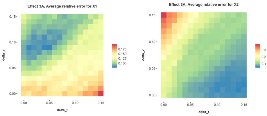
Figure 6: The estimation error in the coefficients for the explanatory factor x1 for Effect 3A as the linear components were varied in E(t) and G(vi) by varying δt and δv respectively.

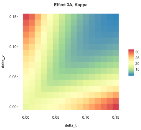
Figure 7: The magnitude of multicolinearity for Effect 3A as measured by kappa as the linear compo- nents were varied in E(t) and G(vi) by varying δt and δv respectively.

In this case, the results will not be symmetric, and this is demonstrated in Figure 8. Furthermore, Figure 8 is affected by censoring affects as defaulted accounts are no longer observed.

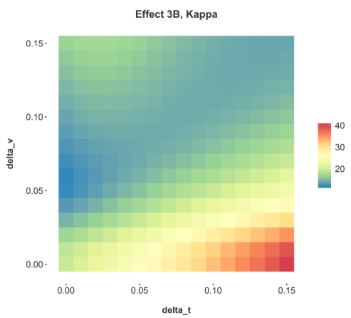
Figure 8: The magnitude of multicolinearity for Effect 3 as measured by kappa as the linear components were varied in E(t) and G(vi) by varying δt and δv respectively.

Comparing Effects 3A and 3B shows that we cannot easily predict how the linear specification error will be expressed when estimating the coefficients. As with any multicolinear situation, the estimation errors will be sensitive to minor variations in the data.

4 Conclusion

those constraints are not explicitly known, we cannot be certain if the obtained stress test model is either under or over sensitive to economic factors, as is possible in the presence of the linear trend specification problem.

We also learn from APC models that the nonlinear components of the age, vintage, and time functions are fully estimable. For stress test models, this means that if we have enough history, at least one full economic cycle but preferably more, then the desired macroeconomic sensitivities are confined in the nonlinear components. The numerical experiments here confirm that given enough data over calendar time and loan age, all these methods almost always provide effective solutions, because the linear trends are approximately zero.

However, in real world applications we rarely have enough data relative to these cycles. For loan portfolios, that could be 20 years minimum. For wine analysis, 40 years might be required for stability [9]. In all these examples, we are also assuming that the underlying system is stable for that period, meaning no changes in business practices or consumer behavior. Therefore, we need to assume that multicollinearity is Cox PH analysis is always present.

For a credit risk analyst who wishes to use the Cox model or an organization with a history of use, the primary advice is to switch from the partial likelihood estimator to a logistic regression or Poisson regression approach. By using an estimator that explicitly includes all of the model components including the hazard function, any multicollinearity problem can be directly tested and addressed.

Solving the collinearity problem will include a review of possible frailty that could distort the shape of the hazard function and embedded trends in the explanatory factors caused when modeling fractions of an economic cycle. If the hazard function can be refined and fixed, then residual multicollinearity among the explanatory factors can be addressed via some of the usual techniques [30, 1], assuming that the estimated hazard function is included as a fixed offset to the estimation. These solutions are identical to those employed in APC models, further demonstrating the parallels between the two approaches.

References

• [1] Anish Agarwal, Devavrat Shah, Dennis Shen, and Dogyoon Song. On robustness of principal component regression. Advances in Neural Information Processing Systems, 32, 2019.
• [2] P.D. Allison and SAS Institute. Survival Analysis Using the SAS System: A Practical Guide. SAS Institute, 1995.
• [3] Borgan O. Gill R.D. Andersen, P.K. and N. Keiding. Statistical Models Based on Counting Processes. Springer-Verlag, New York, 1993.
• [4] G Andreeva, J Ansell, and J Crook. Modelling profitability using survival combination scores. European Journal of Operational Research, 183(3):1537–1549, 2007.
• [5] Theodor A Balan and Hein Putter. A tutorial on frailty models. Statistical methods in medical research, 29(11):3424–3454, 2020.
• [6] T. Bellotti and J.N. Crook. Credit scoring with macroeconomic variables using survival analysis. 60:1699–1707, 2009.
• [7] Joseph L. Breeden. Testing retail lending models for missing cross-terms. Journal of Risk Model Validation, 4(4), 2010.
• [8] Joseph L. Breeden. Reinventing Retail Lending Analytics: Forecasting, Stress Testing, Capital and Scoring for a World of Crises, 2nd Impression. Risk Books, London, 2014.
• [9] Joseph L Breeden. How sample bias affects the assessment of wine investment returns. Journal of Wine Economics, 17(2):127–140, 2022.
• [10] Joseph L. Breeden and Sisi Liang. Auction-price dynamics for fine wines from age-period-cohort models. Journal of Wine Economics, 12(2):173–202, 2017.
• [11] Joseph L. Breeden, Lyn C. Thomas, and John McDonald III. Stress testing retail loan portfolios with dual-time dynamics. Journal of Risk Model Validation, 2(2):43 – 62, 2008.
• [12] N. E. Breslow. Discussion following regression models and life tables by D. R. Cox. Journal of the Royal Statistical Society, Series B (Methodological), 34(2):187–220, 1972.
• [13] N.E. Breslow and N.E. Day. Statistical Methods in Cancer Research: The analysis of case-control studies. IARC scientific publications. International Agency for Research on Cancer, 1984.
• [14] Glenyth Caragata Nasvadi and Andrew Wister. Do restricted driver’s licenses lower crash risk among older drivers? a survival analysis of insurance data from british columbia. The Gerontologist, 49(4):474–484, 2009.
• [15] J. Cohen, S.G.W.L.S.A. Patricia Cohen, Routledge, P. Cohen, S.G. West, L.S. Aiken, Ebooks Corporation, and J.R. Cohen. Applied Multiple Regression/correlation Analysis for the Behavioral Sciences. Number v. 1 in Applied Multiple Regression/correlation Analysis for the Behavioral Sciences. L. Erlbaum Associates, 2003.
• [16] David Collett. Modelling Binary Data, 2nd Edition. Chapman and Hall/CRC, 2002.
• [17] E. R. Cook and L. A. Kairiukstis. Methods of Dendrochronology. Kluwer Academic Publishers, Dordrecht, Netherlands, 1990.
• [18] Bendix Carstensen Steno Diabetes Center Copenhagen. Who needs the cox model anyway. Stat Med, 31:1074–1088, 2012.
• [19] Federal Deposit Insurance Corporation. Supervisory guidance on implementing Dodd-Frank Act company-run stress tests for banking organizations with total consolidated assets of more than $10 billion but less than $50 billion. Technical report, Federal Deposit Insurance Corporation, March 2014.
• [20] D. R. Cox. Regression models and life-tables. Journal of the Royal Statistical Society. Series B (Methodological), 34(2):187–220, 1972.
• [21] D. R. Cox and D. O. Oakes. Analysis of Survival Data. Chapman and Hall, London, 1984.
• [22] Scott A Czepiel. Maximum likelihood estimation of logistic regression models: theory and implementation. Available at czep. net/stat/mlelr. pdf, 83, 2002.
• [23] J. Durbin and G. S. Watson. Testing for serial correlation in least squares regression. Biometrika, 37:409–428, 1950.
• [24] VT Farewell. Some results on the estimation of logistic models based on retrospective data. Biometrika, 66(1):27–32, 1979.
• [25] Federal Reserve Board. Comprehensive capital analysis and review 2015: Summary instructions and guidance. Technical report, Board of Governors of the Federal Reserve System, August, Washington, October 2014.
• [26] Financial Accounting Standards Board. Financial InstrumentsCredit Losses (Subtopic 825-15). Financial Accounting Series, December 20 2012.
• [27] T.R. Fleming and D.P. Harrington. Counting Processes and Survival Analysis. Wiley, New York, 1991.
• [28] Mitchell H. Gail, Jay H. Lubin, and Lawrence V. Rubinstein. Likelihood calculations for matched case-control studies and survival studies with tied death times. Biometrika, 68(3):703–707, 1981.
• [29] Norval D. Glenn. Cohort Analysis, 2nd Edition. Sage, London, 2005.
• [30] Arthur E Hoerl and Robert W Kennard. Ridge regression: applications to nonorthogonal problems. Technometrics, 12(1):69–82, 1970.
• [31] T R Holford. The estimation of age, period and cohort effects for vital rates. Biometrics, 39:311–324, 1983.
• [32] Theodore Holford. Encyclopedia of Statistics in Behavioral Science, chapter Age-Period-Cohort Analysis. Wiley, 2005.
• [33] IASB. IFRS 9 financial instruments. Technical report, IFRS Foundation, 2014.
• [34] J. F. Lawless. Regression methods for poisson process data. Journal of the American Statistical Association, 82(399):808–815, 1987.
• [35] G. M. Ljung and G. E. P. Box. On a measure of a lack of fit in time series models. Biometrika, 65(2):297–303, 1978.
• [36] W.M. Mason and S. Fienberg. Cohort Analysis in Social Research: Beyond the Identification Problem. Springer, 1985.
• [37] Stephen Reid and Rob Tibshirani. Regularization paths for conditional logistic regression: the clogitl1 package. Journal of statistical software, 58(12), 2014.
• [38] Jian-Jian Ren and Mai Zhou. Full likelihood inferences in the cox model: an empirical likelihood approach. Annals of the Institute of Statistical Mathematics, 63(5):1005–1018, Oct 2011.
• [39] Volker Schmid and Leonhard Held. Bayesian age-period-cohort modeling and prediction - bamp. Journal of Statistical Software, Articles, 21(8):1–15, 2007.
• [40] Y. Yang and K.C. Land. Age-Period-Cohort Analysis. Taylor and Francis, Boca Raton, 2014.